Earth’s Energy Imbalance

Fig. 1.  12-month running-mean of Earth’s energy imbalance, based on CERES satellite data for EEI change normalized to 0.71 W/m2 mean for July 2005 – June 2015 based on in situ data.

Earth’s Energy Imbalance and Climate Response Time

22 December 2022

James Hansen, Makiko Sato, Norman Loeb, Leon Simons, Karina von Schuckmann

Our judicious choice of graphs for Global Warming in the Pipeline[1] (submitted to Oxford Open Climate Change, available here with an added list of acronyms) squeezed out a graph of Earth’s energy imbalance (EEI, Fig. 1 above). EEI is the net gain (or loss) of energy by the planet, i.e., the difference between absorbed solar energy and emitted thermal (heat) radiation. EEI is the basic diagnostic informing us where global climate is headed. As long as more energy is coming in than going out, i.e., as long as EEI is positive, Earth will continue to get hotter.

EEI is hard to measure, a small difference between two large quantities (Earth absorbs and emits about 240 W/m2 averaged over the entire planetary surface), but the change of EEI is well-measured from space.[2] Absolute calibration is obtained from the change of heat in the heat reservoirs, mainly the global ocean, over a period of at least a decade, as required to reduce error due to the finite number of places that the ocean is sampled.[3].

EEI varies from year-to-year (Fig. 1), largely because global cloud amount varies with weather and ocean dynamics, but averaged over several years, EEI tells us what is needed to stabilize climate.[4] When JEH gave a TED talk 10 years ago, EEI was about 0.6 W/m2, averaged over six years (that may not sound like much, but it equals the energy in 400,000 Hiroshima atomic bombs per day, every day). Now, it appears, EEI has approximately doubled, to more than 1 W/m2. The reasons, discussed in our paper, mainly being increased growth rate of greenhouse gases (GHGs) and a reduction of human-made aerosols (fine particles in the air that reflect sunlight and cool the planet). We will discuss practical implications of the planetary energy imbalance further below.

Failure of governments to take actions required to stabilize climate is due in part to climate’s delayed response. If the full (equilibrium) climate impact of fossil fuel burning occurred immediately, we likely would have acted more aggressively to limit climate change. On the other hand, the delayed response is useful, if we use the time wisely and take actions to limit the ultimate climate change. Thus, it is important to have a good understanding of climate response time.

Climate response time. The Charney study[5] in 1979 focused on the equilibrium climate sensitivity (ECS) to a CO2 doubling (2×CO2), an idealized gedanken experiment in which the atmosphere and ocean respond to 2×CO2 but other climate variables such as ice sheet size and vegetation are fixed. Charney’s ECS thus includes only “fast” feedbacks such as water vapor, clouds and sea ice. Charney concluded that the fast-feedback 2×CO2 ECS was 3 ± 1.5°C, but noted: “However, we believe it is quite possible that the capacity of the intermediate waters of the ocean to absorb heat could delay the estimated warming by several decades.”

Charney didn’t mention that the delay is a strong function of ECS. The physics is straightforward. Most fast feedbacks come into play not in response to the climate forcing, but in response to global temperature change. Thus, if the climate system’s thermal inertia is fixed (say the heat capacity of the ocean’s well-mixed upper layer), the delay increases linearly with ECS (for example, the delay is twice as long for ECS = 4°C as for ECS = 2°C). However, as the mixed layer warms, it exchanges water with the deeper ocean, slowing the mixed layer warming. If mixing into the deeper ocean is approximated as diffusive, surface temperature response time is proportional to the square of ECS.[6]

Real-world ocean heat uptake is more complex than diffusion. Atmosphere-ocean GCMs (global climate models) can provide a more reliable climate response time, if they realistically simulate ocean dynamics and mixing. In 2008, one of us (JEH) suspected that the GISS (Goddard Institute for Space Studies) GCM mixed heat too efficiently into the deep ocean; in 100 years, global surface temperature achieved only 60% of its equilibrium response. For his “Bjerknes” presentation[7] at the 2008 American Geophysical Union meeting, he requested 2×CO2 GCM results from the three leading modeling groups in the world; all of them[8] graciously provided 2×CO2 simulations. All three models had a response time as slow or slower than that of the GISS GCM. This did not resolve the matter; suspicion remained that all these models mixed heat downward more efficiently than the real world. More attention to the temporal response to an instant CO2 doubling seemed warranted. For one thing, that response constitutes a Green’s function,[7] which facilitates study of climate problems by people who do not have access to or do not wish to run a global GCM.

However, aerosols were the issue of special concern in this AGU discussion. The suspicion was that excessive, unrealistic, mixing of heat into the deep ocean caused climate modelers to underestimate the climate forcing by human-made aerosols.

Ocean mixing and aerosols. If ocean models mix heat downward too rapidly, why do GCMs yield realistic global warming over the past century? They can do it by understating aerosol cooling because the aerosol climate forcing is unmeasured. Excessive ocean mixing reduces warming at the ocean surface. For that reason, climate models do not need as much of the process that actually reduces warming in the real world: human-made aerosols. It’s easy to achieve a too-small aerosol forcing: omit or underestimate the aerosol effect on clouds.

The aerosol issue continues today. How large is the aerosol forcing? Is the aerosol amount now declining,[9] causing an acceleration of global warming? In other words, is the payment for our Faustian aerosol bargain[10] coming due? Those questions are addressed in our Pipeline paper,[1] but quantitative understanding requires knowledge of climate response time, and that requires an ability to simulate global ocean dynamics and mixing realistically.

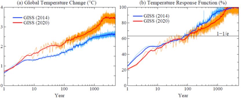
Fig. 2. (a) Global mean surface temperature response to instant CO2 doubling, and (b) normalized response function (percent of final change). Thick lines are smoothed[11] results.

A newer GISS model. Max Kelley revamped the GISS ocean model. Ocean mixing was improved by use of a high-order advection scheme,[12] finer vertical resolution (40 layers), updated mesoscale eddy parameterization, and correction of errors in the ocean modeling code. The newer GCM[13] has improved internal variability, including the Madden-Julian Oscillation (MJO), El Nino Southern Oscillation (ENSO) and Pacific Decadal Oscillation (PDO), although the spectral signature of the ENSO-like variability is unrealistic and its amplitude is excessive, as shown by the size of oscillations in Fig. 2, discussed below. Ocean mixing in GISS (2020) may still be a bit excessive in the North Atlantic, where the model’s simulated penetration of CFCs is greater than observed.[14]

We can learn something by comparing successive versions of the GISS model, even if portions of the physics in the model are still unrealistic. Specifically, we use two model versions: GISS (2014) and GISS (2020),[15] both described by Kelley et al. (2020).[12] Clouds are still parameterized crudely in the GISS (2020) model, but with a change that allows inference of a remarkable relation between clouds and the ocean’s response time. The cloud change is in the glaciation parameterization at cloud temperatures with mixed phase cloud particles. The GISS (2014) model has an unrealistically small portion of supercooled liquid drops, while the (2020) model errs in the opposite sense: the fraction of cloud particles that are supercooled drops is too large.

Climate response time. The surprising effect of cloud particle microphysics on the ocean, in the end, is easy to understand. In the “Bjerknes” discussion it was assumed that the lag in climate response depended only on the ocean’s effective thermal inertia (thus on ocean mixing) and ECS. Therefore, based on evidence that the GISS (2020) model had largely eliminated excessive, unrealistic, ocean mixing, we expected a faster surface temperature response to a 2×CO2 forcing – but that is not what we found (Fig. 2). Instead, as a fraction of the equilibrium response, the newer model is slightly slower than the old model (Fig. 2b). Both models need 100 years to reach within 1/e of equilibrium warming, i.e., 63% of the equilibrium response. There are two reasons for the slow response of the newer model, one that is obvious and one that is more interesting.

Initially the two models warm at the same rate (Fig. 2a), as expected because stronger feedback in the GISS (2020) model only comes into play as warming occurs. Speedup of surface warming in GISS (2020) due to reduced ocean mixing is partly offset by the higher ECS of the newer model, which increases the time needed to reach equilibrium. The more interesting difference between the models becomes apparent when we compare the EEI response functions of the two models (Fig. 3).

Fig. 3. (a) Earth’s energy imbalance (EEI) for 2×CO2, and (b) EEI response function.

Earth’s energy imbalance in the newer model decreases rapidly, by one-third, in response to 2×CO2 forcing (Fig. 3a). EEI defines the rate heat is pumped into the ocean, so smaller EEI implies longer time for the ocean to reach its new equilibrium. This quick drop of EEI is ultrafast, almost instant, in response to the forcing (“fast” feedbacks occur rapidly in response to temperature change, but the temperature change occurs over a millennium, Fig. 2a). Surely, for want of an alternative, this ultrafast feedback must be a cloud change induced by the 2×CO2 radiative forcing.

Indeed, the cloud physics community is aware of quick cloud response to radiative forcing. Andrews et al.,[16] Zelinka et al.[17] and Kamae et al.[18] review rapid cloud adjustments separate from global temperature-mediated changes. Clouds can respond to radiative forcing, e.g., via effects on cloud particle phase, cloud cover, cloud albedo and precipitation.[19] This raises the question of whether it is more helpful to think of this quick response as an adjustment – and incorporate it in an adjusted climate forcing – or as an ultrafast feedback. Rapid response of stratospheric temperature to CO2 change, e.g., is included in an adjusted forcing. This is useful: the adjusted forcing then yields a global temperature change consistent with other forcings of similar magnitude. All climate models with realistic radiation calculations find similar forcing after adjusting for stratospheric change.

In contrast, it is unlikely that cloud adjustments will be similar among all climate models because the cloud physics treatments vary widely and are still being developed. We suggest that there is merit in describing the cloud adjustment as an ultrafast climate feedback for sake of interpreting temperature (Fig. 2) and EEI (Fig. 3) responses to a climate forcing. The nearly instant one-third reduction of EEI in the GISS (2020) model should not be interpreted as the clouds causing a smaller forcing, which would leave the impression that the expected climate change is reduced. On the contrary, it is likely that clouds cause ECS to be larger (Fig. 2a), but the clouds’ ultrafast feedback can tend to fool us by slowing down the rate of ocean warming, thus increasing the response time of global climate.

Climate response functions. EEI reaches 63% response (return toward equilibrium) in only 10 years (Fig. 3b) in the GISS (2020) model. This fast response of EEI decreases energy flux into the ocean. But is this fast response realistic? The EEI response time varies from ~10 years in the GISS (2020) model to ~50 years in GISS (2014), perhaps because the division of cloud particles among water and ice are on opposite sides of reality in these two models (Fig. 1 of Kelley, et al.).[13] The exact cloud changes that cause this behavior in the models can be determined from a large set of brief GCM runs, each with 2×CO2 added at a different point on a control run of the GCM, thus defining cloud changes and other diagnostic quantities to an arbitrary accuracy.

Several research groups are working on inclusion of detailed cloud microphysics in GCMs. It would be useful if the temperature and EEI response functions were provided for all models. Given that real-world ECS is at least ~4°C for 2×CO2, there is probably more amplifying cloud feedback in the real world than in the GISS (2020) model. How much of the feedback is ultrafast, as opposed to fast? That partition determines the degree to which Earth’s energy imbalance is a measure of the climate forcing reduction required to stabilize climate, as shown in the Pipeline paper.

Andrews et al. (2012)[16] estimate that rapid cloud adjustment contributes 0.8°C of the 4.4°C 2×CO2 equilibrium response of a Hadley Centre climate model, implying that their model also has a large ultrafast response. This is consistent with a substantial ultrafast response, but attribution to specific cloud changes would be aided by diagnostic study as suggested above.

Summary. Now let’s return to discussion of Fig. 1, Earth’s energy imbalance (EEI). In its own right, EEI is the single most important diagnostic quantity characterizing the status of climate change, the prospects for continued global warming, stabilization of global temperature, or cooling of the planet. EEI has large natural variability on time scales of a few years and even longer time scales, mainly because clouds are sensitive to fluctuations of weather patterns and ocean dynamics. Thus, we need more time to access the magnitude and significance of the increase of EEI over the past decade.

However, we can say with confidence that EEI increased in the past decade, an increase consistent with independent evidence that the growth rate of human-made climate forcing increased. Increased EEI is the basis for our projection that global warming will accelerate by as much as 50-100% in the few decades following 2010 (Fig. 4). The length of this period of accelerated warming will depend on the path humanity follows in its continuing changes of atmospheric composition.

Fig. 4.  Global surface temperature relative to 1880-1920 mean.

Our pragmatic evaluation based on real-world data is an essential antidote to assessments associated with the annual United Nations COP (Conference of the Parties) meetings, which give the impression that much progress is being made and it is still feasible to limit global warming to as little as 1.5°C. Once governments and the public understand Fig. 1, they should recognize it as a wake-up call about the untenable situation that we are creating for young people.

Thus, it is crucial that the remarkable observations that allowed construction of Fig. 1 are continued and improved – which is a greater challenge than governments may be aware of. Precise observations are needed from space and throughout the global ocean.

The measurements of Earth’s radiation budget from space were largely a product of the burst of government spending in the 1990s on NASA’s Earth Observing System. As yet there are no firm adequate plans for long-term continuation of these observations. NASA tends to think of itself as an agency that develops scientific and instrumental techniques, while continued long-term observations should be carried on by others. However, in the case of climate change, long-term observations are the science. It is crucial that NASA make plans to continue these essential measurements.

Measurements in the ocean are equally important. The Argo program that distributed about 4,000 autonomous, deep-diving floats around the world ocean needs to be continued and enhanced. More measurements are needed especially in the polar regions where some of the most significant climate changes are beginning to occur, changes that will affect the entire planet. The U.S. National Atmospheric and Oceanic Administration (NOAA) has provided a large fraction of the Argo floats, but many other nations contribute; the programs should continue their development.

It will be noted that we are using EEI as a crude, indirect, way to assess changes in global aerosols, and the climate forcing caused by aerosols that occurs principally via effects on clouds. It would be much better if we also had more direct measurement of aerosol (and other) climate forcings, as was proposed for a Climsat mission decades ago.[20] Although such a monitoring mission was considered to be outside the scope of NASA’s science program, it would be no less valuable today. One of the measurement techniques proposed for Climsat, high-precision polarimetry, will be tested on NASA’s PACE (Plankton, Aerosol, Cloud, ocean Ecosystem) mission[21] scheduled for launch in 2024.

Twitter-World “science.” We have been told that a bizarre criticism of the Pipeline paper appeared on Twitter, concluding that our paper was “wrong,” because we did not consider that GHGs in the atmosphere would soon be declining as human emissions decrease and the ocean and atmosphere absorb the human-made increase of GHGs.

We hope that even the non-scientist can see through such thinking. When Charney defined the gedanken problem: what is the equilibrium climate sensitivity (ECS) to 2×CO2 forcing, he knew that keeping CO2 fixed at that level and fixing certain boundary conditions such as ice sheet size was an idealized situation designed to help develop an understanding of climate change and climate feedbacks. Our conclusion that ECS is at least ~4°C, near the upper end of Charney’s estimated range, refers to that specific problem. Our study does more than that, however, we also address the delay in the climate response caused by the ocean’s thermal inertia (Fig. 2). With the help of Earth’s paleoclimate history, we also address the question: what is Earth System Sensitivity (ESS) for the idealized case in which 2×CO2 forcing is kept constant until all fast and slow feedbacks are allowed to reach equilibrium. The answer we find is close to 10°C, for CO2 forcing alone. If we include the negative forcing by today’s aerosols, the response may be as low as 6-7°C, but ESS is ~10°C.

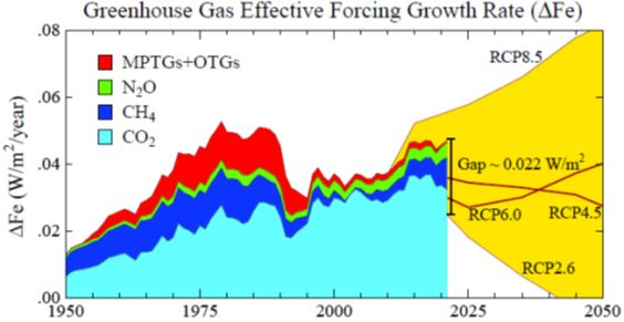
Fig. 5. Update[22] of annual growth of climate forcing by GHGs, including part of O3 forcing via the efficacy of CH4 forcing (cf. Supporting Material in Pipeline paper). MPTG and OTG are Montreal Protocol and Other Trace Gases. RCP2.6 is a scenario designed to keep global warming below 2°C.

Of course, we are not saying that such temperatures will occur in the near term – we would need to wait until ice sheets shrink to a much smaller size and the global deep ocean warms. However, on the near-term we are likely to see an acceleration of warming (Fig. 4). This raises the question of whether the United Nations COP and its advisory process are working well. It is fine to provide scenarios with rapid reduction of the human-made climate forcing, such as scenario RCP2.6 (Fig. 5), but we should not allow policymakers to view the world through unrealistic rose-colored glasses that leave young people to bear the burden of our ignorance.

Twittering can be fun. Perhaps there is merit in twittering things that build up a large number of “followers” and help sell books that might help inform the public, but that information needs to be valid, if it is to be useful. We hope that there is also support for an approach that focuses on advancing the science, which necessarily means avoiding get caught up in Twitter banter.

[1] Hansen, J.E., M. Sato, L. Simons, L.S. Nazarenko, K. von Schuckmann, N.G. Loeb, M.B. Osman, P. Kharecha, Q. Jin, G. Tselioudis, A. Lacis, R. Ruedy, G. Russell, J. Cao, J. Li, Global Warming in the Pipeline, submitted to Oxford Open Climate Change.

[2] Loeb, N. G., Johnson, G. C., Thorsen, T. J., Lyman, J. M., Rose, F. G., & Kato, S., Satellite and ocean data reveal marked increase in Earth’s heating rate, Geophys. Res. Lett. 48, e2021GL093047, 2021.

[3] von Schuckmann, K., L. Cheng, M.D. Palmer, J. Hansen et al.: Heat stored in the Earth system: where does the energy go?, Earth System Science Data 12, 2013-2041, doi:10.5195/essd-12-2013-2020, 2020.

[4] Sentinel for the Home Planet, 7 September 2020 Climate Science, Awareness and Solutions communication.

[5] Charney, J., Arakawa, A., Baker, D., Bolin, B., Dickinson, R., Goody, R., Leith, C., Stommel, H. and Wunsch, C.: Carbon Dioxide and Climate: A Scientific Assessment, Natl. Acad. Sci. Press, Washington, DC, 33p, 1979.

[6] Hansen, J., G. Russell, A. Lacis, I. Fung, D. Rind, and P. Stone: Climate response times: dependence on climate sensitivity and ocean mixing. Science, 229, 857-859, 1985.

[7] Hansen J Climate Threat to the Planet, American Geophysical Union, San Francisco, California, 17 December 2008, http://www.columbia.edu/~jeh1/2008/AGUBjerknes20081217.pdf. (3 December 2022, date last accessed).

[8] Tom Delworth (NOAA Geophysical Fluid Dynamics Laboratory), Gokhan Danabasoglu (National Center for Atmospheric Research), and Jonathan Gregory (UK Hadley Centre) provided long 2×CO2 runs of their GCMs.

[9] Quaas, J., H. Jia, C. Smith, A.L. Albright, W. Aas, N. Bellouin, O. Boucher, M.Doutriaux-Boucher, P.M. Forster, D. Grosvenor, S. Jenkins, Z. Klimont, N.G. Loeb, X. Ma, V. Naik, F. Paulot, P. Steir, M. Wild, G. Myhre and M. Schulz: Robust evidence for reversal of the trend in aerosol effective climate forcing, Atmos. Chem. Phys. 22, 12,221-12,239, 2022.

[10] Hansen, J., 2009: Storms of My Grandchildren, Bloomsbury, New York, 320 pages.

[11] Yr 1 (no smoothing), yr 2 (3-yr mean), yr 3-12 (5-yr mean), yr 13-300 (25-yr mean), yr 301-5000 (101-yr mean).

[12] Prather, M. J.: Numerical advection by conservation of second order moments. J. Geophys, Res. 91, 6671–6680, 1986.

[13] Kelley, M., G.A. Schmidt, L. Nazarenko, S.E. Bauer, R. Ruedy, G.L. Russell, et al., GISS-E2.1: Configurations and climatology. J. Adv. Model. Earth Syst., 12, no. 8, e2019MS002025, 2020.

[14] Romanou, A., Marshall, J., Kelley, M., & Scott, J., Role of the ocean's AMOC in setting the uptake efficiency of transient tracers. Geophysical Research Letters, 44, 5590–5598, 2017.

[15] The GISS (2014) model is labeled as GISS-E2-R-NINT and GISS (2020) as GISS-E2.1-G-NINT in published papers, where NINT (noninteractive) signifies that the models use specified GHG and aerosol amounts.

[16] Andrews,T., Gregory, J.M., Forster, P.M., and Webb, M.J.: Cloud adjustment and its role in CO2 radiative forcing and climate sensitivity: a review. Surv. Geophys. 23, 619-635, 2012.

[17] Zelinka, M.D., S.A. Klein, K.E. Taylor, T. Andrews, M.J. Webb, J.M. Gregory and P.M. Forster: Contributions of different cloud types to feedbacks and rapid adjustments in CMIP5, J. Clim. 26(14), 5007-5027, 2013.

[18] Kamae, Y., M. Watanabe, T. Ogura, M. Yoshimori and H. Shiogama: Rapid adjustments of cloud and hydrological cycle to increasing CO2: a review, Curr. Clim. Chan. Rep 1, 103-113, 2015.

[19] Zelinka, M.D., T.A. Myers, D.T. McCoy, S.Po-Chedley, P.M. Caldwell, P. Ceppi, S.A. Klein and K.E. Taylor, Causes of higher climate sensitivity in CMIP6 models, Geophys. Res. Lett. 47, e2019GL085782, 2020.

[20] Hansen, J., W. Rossow and I. Fung, Long-Term Monitoring of Global Climate Forcings and Feedbacks, NASA CP-3234, 91 pages, 1993.

[21] Plankton, Aerosol, Cloud, ocean Ecosystem (PACE) satellite mission.

[22] Hansen, J. and M. Sato. Greenhouse gas growth rates. Proc. Natl. Acad. Sci. 101, 16109-16114, 2004.