https://arxiv.org/abs/2212.04474
Physics > Atmospheric and Oceanic Physics
[Submitted on 8 Dec 2022 (v1), last revised 12 Dec 2022 (this version, v2)]
Global warming in the pipeline
James E. Hansen (1), Makiko Sato (1), Leon Simons (2), Larissa S. Nazarenko (3 and 4), Karina von Schuckmann (5), Norman G. Loeb (6), Matthew B. Osman (7), Pushker Kharecha (1), Qinjian Jin (8), George Tselioudis (3), Andrew Lacis (3), Reto Ruedy (3 and 9), Gary Russell (3), Junji Cao (10), Jing Li (11) ((1) Climate Science, Awareness and Solutions, Columbia University Earth Institute, New York, NY, USA, (2) The Club of Rome Netherlands, 's-Hertogenbosch, The Netherlands, (3) NASA Goddard Institute for Space Studies, New York, NY, USA, (4) Center for Climate Systems Research, Columbia University Earth Institute, New York, NY, USA, (5) Mercator Ocean International, Ramonville St.-Agne, France, (6) NASA Langley Research Center, Hampton, VA, USA, (7) Department of Geosciences, University of Arizona, Tucson, AZ, USA, (8) Department of Geography and Atmospheric Science, University of Kansas, Lawrence, KS, USA, (9) Business Integra, Inc., New York, NY, USA, (10) Institute of Atmospheric Physics, Chinese Academy of Sciences, Beijing, China, (11) Department of Atmospheric and Oceanic Sciences, School of Physics, Peking University, Beijing, China)
Improved knowledge of glacial-to-interglacial global temperature change implies that fast-feedback equilibrium climate sensitivity is at least ~4°C for doubled CO2 (2xCO2), with likely range 3.5-5.5°C. Greenhouse gas (GHG) climate forcing is 4.1 W/m2 larger in 2021 than in 1750, equivalent to 2xCO2 forcing. Global warming in the pipeline is greater than prior estimates. Eventual global warming due to today's GHG forcing alone -- after slow feedbacks operate -- is about 10°C. Human-made aerosols are a major climate forcing, mainly via their effect on clouds. We infer from paleoclimate data that aerosol cooling offset GHG warming for several millennia as civilization developed. A hinge-point in global warming occurred in 1970 as increased GHG warming outpaced aerosol cooling, leading to global warming of 0.18°C per decade. Aerosol cooling is larger than estimated in the current IPCC report, but it has declined since 2010 because of aerosol reductions in China and shipping. Without unprecedented global actions to reduce GHG growth, 2010 could be another hinge point, with global warming in following decades 50-100% greater than in the prior 40 years. The enormity of consequences of warming in the pipeline demands a new approach addressing legacy and future emissions. The essential requirement to "save" young people and future generations is return to Holocene-level global temperature. Three urgently required actions are: 1) a global increasing price on GHG emissions, 2) purposeful intervention to rapidly phase down present massive geoengineering of Earth's climate, and 3) renewed East-West cooperation in a way that accommodates developing world needs.
Comments: |
48 pages, 27 figures. Correction of formatting error on page 21, which messed up placement of all following figures |
Subjects: |
Atmospheric and Oceanic Physics (physics.ao-ph) |
Cite as: |
arXiv:2212.04474 [physics.ao-ph] |
|
(or arXiv:2212.04474v2 [physics.ao-ph] for this version) |
|
Submission history
From: James Hansen [view email]
[v1] Thu, 8 Dec 2022 18:48:43 UTC (2,063 KB)
[v2] Mon, 12 Dec 2022 18:55:10 UTC (2,062 KB)
https://arxiv.org/pdf/2212.04474v1
2212.04474v1.pdf
Global warming in the pipeline
James E. Hansen, 1 Makiko Sato, 1 Leon Simons, 2 Larissa S. Nazarenko, 3,4 Karina von
Schuckmann, 5 Norman G. Loeb, 6 Matthew B. Osman, 7 Pushker Kharecha, 1 Qinjian Jin, 8
George Tselioudis, 3 Andrew Lacis, 3 Reto Ruedy, 3,9 Gary Russell, 3 Junji Cao, 10 Jing Li 11
* Correspondence: James E. Hansen <jeh1@columbia.edu>
ABSTRACT
Improved knowledge of glacial-to-interglacial global temperature change implies that fast-
feedback equilibrium climate sensitivity is at least ~4°C for doubled CO 2 (2×CO 2 ), with likely
range 3.5-5.5°C. Greenhouse gas (GHG) climate forcing is 4.1 W/m 2 larger in 2021 than in
1750, equivalent to 2×CO 2 forcing. Global warming in the pipeline is greater than prior
estimates. Eventual global warming due to today’s GHG forcing alone – after slow feedbacks
operate – is about 10°C. Human-made aerosols are a major climate forcing, mainly via their
effect on clouds. We infer from paleoclimate data that aerosol cooling offset GHG warming for
several millennia as civilization developed. A hinge-point in global warming occurred in 1970
as increased GHG warming outpaced aerosol cooling, leading to global warming of 0.18°C per
decade. Aerosol cooling is larger than estimated in the current IPCC report, but it has declined
since 2010 because of aerosol reductions in China and shipping. Without unprecedented global
actions to reduce GHG growth, 2010 could be another hinge point, with global warming in
following decades 50-100% greater than in the prior 40 years. The enormity of consequences of
warming in the pipeline demands a new approach addressing legacy and future emissions. The
essential requirement to "save" young people and future generations is return to Holocene-level
global temperature. Three urgently required actions are: 1) a global increasing price on GHG
emissions, 2) purposeful intervention to rapidly phase down present massive geoengineering of
Earth’s climate, and 3) renewed East-West cooperation in a way that accommodates developing
world needs.
Climate Science, Awareness and Solutions, Columbia University Earth Institute, New York, NY, USA
2 The Club of Rome Netherlands, ‘s-Hertogenbosch, The Netherlands
3 NASA Goddard Institute for Space Studies, New York, NY, USA
4 Center for Climate Systems Research, Columbia University Earth Institute, New York, NY, USA
5 Mercator Ocean International, Ramonville St.-Agne, France
6 NASA Langley Research Center, Hampton, VA, USA
7 Department of Geosciences, University of Arizona, Tucson, AZ, USA
8 Department of Geography and Atmospheric Science, University of Kansas, Lawrence, KS, USA
9 Business Integra, Inc., New York, NY, USA
10 Institute of Atmospheric Physics, Chinese Academy of Sciences, Beijing, China
11 Department of Atmospheric and Oceanic Sciences, School of Physics, Peking University, Beijing, China
INTRODUCTION
It has been known since the 1800s that infrared-absorbing (greenhouse) gases (GHGs) warm
Earth’s surface and that the abundance of GHGs changes naturally as well as from human
actions. 1,2 Roger Revelle wrote in 1965 that we are conducting a “vast geophysical experiment”
by burning fossil fuels that accumulated in Earth’s crust over hundreds of millions of years. 3
Carbon dioxide (CO 2 ) in the air is now increasing and already has reached levels that have not
existed for millions of years, with consequences that have yet to be determined. Jule Charney led
a study in 1979 by the United States National Academy of Sciences that concluded that doubling
of atmospheric CO 2 was likely to cause global warming of 3 ± 1.5°C. 4 Charney added:
“However, we believe it is quite possible that the capacity of the intermediate waters of the
ocean to absorb heat could delay the estimated warming by several decades.”
After U.S. President Jimmy Carter signed the 1980 Energy Security Act, which included a focus
on unconventional fossil fuels such as coal gasification and rock fracturing (“fracking”) to
extract shale oil and tight gas, the U.S. Congress asked the National Academy of Sciences again
to assess potential climate effects. Their Changing Climate report has a measured tone on energy
policy – amounting to a call for research. 5 Was not enough known to caution lawmakers against
taxpayer subsidy of the most carbon-intensive fossil fuels? Perhaps the equanimity was due in
part to a major error: the report assumed that the delay of global warming caused by the ocean’s
thermal inertia is 15 years, independent of climate sensitivity. With that assumption, they
concluded that climate sensitivity for 2×CO 2 is near or below the low end of Charney’s 1.5-
4.5°C range. If climate sensitivity was low and the lag between emissions and climate response
was only 15 years, climate change would not be nearly the threat that it is.
Simultaneous with preparation of Changing Climate, a symposium was held 25-27 October 1982
at Columbia University’s Lamont Doherty Geophysical Observatory, with papers published in
January 1984 as Climate Processes and Climate Sensitivity, a monograph of the American
Geophysical Union. 6 The symposium focused on the ocean’s role in climate change and on
climate change information contained in the paleoclimate record. Paleoclimate data showed that
climate sensitivity is in the range 2.5-5°C for 2×CO 2 , thus at the upper end of Charney’s range.
In turn, this implied that the climate response time to a forcing is of the order of a century, not 15
years. Thus, the concept that a large amount of additional human-made warming is already “in
the pipeline” was introduced. 7 E.E. David, Jr., President of Exxon Research and Engineering, in
his keynote talk at the symposium insightfully noted: “The critical problem is that the
environmental impacts of the CO 2 buildup may be so long delayed. A look at the theory of
feedback systems shows that where there is such a long delay, the system breaks down, unless
there is anticipation built into the loop.” 8
Thus, the danger caused by climate’s delayed response and the need for anticipatory action to
alter the course of fossil fuel development was apparent to scientists and the fossil fuel industry
40 years ago. 9 Yet industry chose to long deny the need to change energy course, 10 and now,
while governments and financial interests connive, most industry adopts a “greenwash” approach
that threatens to lock in perilous consequences for humanity. Scientists will share responsibility,
if we allow governments to rely on goals for future global GHG levels as if targets had meaning
2
in the absence of policies required to achieve them. In the final section of this perspective article,
we discuss actions required to slow down and reverse global warming.
The Intergovernmental Panel on Climate Change (IPCC) was established in 1988 to provide
policymakers with regular scientific assessments on the current state of knowledge about climate
change 11 and almost all nations agreed to the 1992 United Nations Framework Convention on
Climate Change 12 with the objective to avert “dangerous anthropogenic interference with the
climate system,” The current IPCC Working Group 1 report 13 describes shutdown of the
overturning ocean circulations and large sea level rise on the century time scale as “high impact,
low probability” even under extreme GHG growth scenarios. This contrasts with “high impact,
high probability” assessments reached in a paper – hereafter abbreviated Ice Melt – that several
of us published in 2016. 14 Recently, the first author (JEH) of our present paper published a
qualitative description of the decade-long investigation that led to the conclusion that most
climate models are unrealistically insensitive to freshwater injected by melting ice and also that
ice sheet models are unrealistically lethargic in the face of rapid, large climate change. 15
Eelco Rohling, editor-in-chief of Oxford Open Climate Change, invited one of us (JEH) to write
a perspective article on these scientific issues. We had noted in our papers that global warming in
the past century does not imply a unique climate sensitivity because the warming at Earth’s
surface depends on three major unknowns with only two fundamental constraints. Unknowns are
ECS, net climate forcing (because aerosol forcing is unmeasured), and ocean mixing of heat.
Constraints are observed global temperature change and EEI. In our investigation noted above,
we assumed the canonical climate sensitivity 3°C for 2×CO 2 , thus leaving two unknowns and
two constraints. This allowed us to confirm that most climate models mix heat excessively into
the deeper ocean and compensate for this by using a less strong aerosol forcing (less negative)
than real-world aerosols.
A fresh look at this problem is demanded by two recent developments. First, improved analyses
of global temperature during the last glacial maximum and during the prior (Eemian) interglacial
period allow inference that ECS is higher than the canonical estimate. Second, although aerosol
climate forcing remains unmeasured, there is evidence that human-made aerosol amount is on
the decline, implying that acceleration of global warming may be in the offing. We clarify the
physics by use of “response functions” for both global temperature and EEI, which reveal that
climate response time is not simply a function of ocean mixing. We infer that ultrafast cloud
feedbacks affect global temperature and EEI in opposite senses – slowing the warming of the
ocean while speeding up partial restoration of planetary energy balance. We will describe
implications in two papers. This first paper – Global Warming in the Pipeline – focuses on
climate sensitivity, climate response time, and aerosols. The second paper – Sea Level Rise in the
Pipeline – presents evidence that continued warming and increasing ice melt can cause shutdown
of the overturning ocean circulations within decades and large sea level rise within a century.
3
CLIMATE SENSITIVITY
Charney defined an equilibrium climate sensitivity (ECS): the eventual global temperature
change caused by doubled CO 2 in the idealized case in which ice sheets, vegetation and long-
lived GHGs are fixed (except for the specified CO 2 doubling). All other quantities are allowed to
change. The ones deemed most significant – clouds, aerosols, water vapor, snow cover and sea
ice – change rapidly in response to climate change. Thus, the Charney ECS is also called the
“fast feedback” climate sensitivity. Feedbacks can interact in many ways, so their changes are
usually calculated in global climate models (GCMs) that can simulate such interactions. Charney
implicitly assumed that change of the ice sheets on Greenland and Antarctica – which we will
categorize as a “slow feedback” – was not important on the time scale of most public interest.
ECS defined by Charney is a useful concept that helps us understand how human-made and
natural climate forcings affect climate. We must also consider an Earth system sensitivity, 16 ESS,
in which all feedbacks are allowed to respond to a climate forcing. ECS and ESS both depend on
the initial climate state 17,18 and direction (warming or cooling) of climate change, but at the
present climate state – with ice sheets on Antarctica and Greenland – climate should be about as
sensitive in the warmer direction as in the cooler direction. Paleoclimate data indicate that ESS
substantially exceeds ECS, i.e., when feedbacks that Charney kept fixed are allowed to change,
climate sensitivity increases. As Earth warms, ice sheets shrink and the atmosphere contains
more CO 2 , CH 4 and N 2 O, at least on glacial-interglacial time scales.
The time scale of climate feedbacks is crucial, but poorly understood, especially for the unique
human-made forcing. As quantified below, the human-made GHG climate forcing is already 4
W/m 2 , equivalent to 2×CO 2 , and a GHG forcing as large as 8 W/m 2 (equivalent to 4×CO 2 ) is
possible, perhaps likely, within a century. Such forcing is larger than estimates of the forcing that
drove the largest known rapid global warming, the Paleocene Eocene Thermal Maximum
(PETM), 19 which occurred ~56 MyBP. The CO 2 increase that drove PETM global warming was
introduced over a few thousand years. 20 The net human-made climate forcing has been growing
rapidly only since about 1970, i.e., for about half a century, but within another century it could
match or exceed the PETM forcing, while being introduced 20 times faster. There is no known
paleoclimate analogue of such a forcing. In Sea level rise in the Pipeline it will be argued that
such a large, rapid forcing will cause nonlinear growth of ice melt, that excessive small-scale
ocean mixing in most GCMs has caused underestimate of the effect of ice melt on overturning
ocean circulations, that the world is nearing ice melt rates that will affect these circulations, that
increasing ice melt increases Earth’s energy imbalance thus accelerating ice melt and creating
the danger of collapse of the West Antarctic ice sheet on a century time scale. Such increased ice
melt and shutdown of ocean circulations, if they occur, will cool the North Atlantic and Southern
Oceans. That type of cooling is not helpful, as it increases Earth’s energy imbalance and thus the
rate at which energy is pumped into the ocean. The cooling needed to slow and stop global
warming and ice melt requires reducing and eliminating Earth’s energy imbalance caused by the
human-made climate forcing. Despite the danger of transitioning into nonlinear climate change –
indeed, because of that danger – improved understanding of ECS is important. High ECS
increases climate response time and the amount of global warming presently “in the pipeline”
without further increase of climate forcing.
4
If knowledge of ECS was based only on models, it would be difficult to narrow the range of
estimated climate sensitivity – or to have high confidence in any range – because we do not
know how well feedbacks are modeled or even if the models include all significant real-world
feedbacks. Cloud and aerosol interactions are complex, and even small cloud changes can have a
substantial effect. That is why data on Earth’s paleoclimate history are so valuable; they allow us
to compare different equilibrium climate states, knowing that all feedbacks were in operation.
Climate sensitivity estimated at Ewing Symposium
In our paper 7 for the AGU Geophysical Monograph we compared the Last Glacial Maximum
(LGM) with the current interglacial period (the Holocene). We ran GCM simulations introducing
one-by-one LGM surface conditions provided by the CLIMAP project 21 and analyzed the effect
of individual feedbacks on global change. With all CLIMAP surface conditions incorporated in
the GCM – including ice sheet sizes and sea surface temperature (SST) – the calculated global
mean surface temperature was 3.6°C colder in the LGM than in the Holocene. From analysis of
the strength of individual feedbacks, we estimated ECS for 2×CO 2 as 2.5-5°C.
We recognized the potential to get a more certain and accurate evaluation of ECS by using the
fact that Earth had to be in energy balance during the LGM. With CLIMAP surface conditions,
we found that the model Earth was out of energy balance by 2.1 W/m 2 , radiating more energy to
space than it receives from the Sun. Such a large energy imbalance is impossible; averaged over
millennia, the planet had to be in energy balance within less than 0.1 W/m 2 . Earth (i.e., the
climate model with CLIMAP SSTs) was trying to cool off; it would need to cool at least 1-2°C
to achieve energy balance. When we employed CLIMAP’s “maximal extent” ice sheet area –
assuming that maximum ice sheet size was obtained simultaneously on all continents in both
hemispheres – the increased reflection of sunlight only reduced the imbalance to 1.6 W/m 2 .
Something was wrong with either CLIMAP surface conditions or our assumed change of
atmospheric composition between the LGM and today. Indeed, we did not realize that – in
addition to reduced CO 2 – CH 4 and N 2 O were less abundant in the LGM than today. However,
the effect of that change is moderate and the sense is to make the energy imbalance even larger.
A likely explanation was that CLIMAP SSTs were unrealistically warm. We noted independent
evidence for that conclusion, including a then-ongoing study of proxy temperature data by Rind
and Peteet that indicated low latitude CLIMAP SSTs were too warm by as much as 2-3°C. 22
Colder SSTs during the LGM implied a higher climate sensitivity. Our calculated climate forcing
for the Holocene relative to the LGM (due to ice sheet, vegetation and CO 2 change) was almost 6
W/m 2 . Forcing by 2×CO 2 is ~4 W/m 2 , two-thirds of the LGM-to-Holocene forcing, so
CLIMAP’s estimate of 3.6°C temperature change implied an ECS at the low end of the 2.5-5°C
range estimated from our feedback analysis. But if the LGM was cooler – as implied by the
calculated energy imbalance – ECS would be in the upper part of the 2.5-5°C range.
CLIMAP project members would not concede such large errors in LGM SSTs. Therefore, we
concluded only that climate sensitivity was 2.5-5°C for 2×CO 2 . Even so, that range was more
precise and reliable than climate models alone can ever provide. Today, advanced techniques for
analysis allow more definitive assessment of climate sensitivity. Tierney et al. 23 used a large
collection of geochemical proxies for SST constrained by isotope measurements and climate
5
change patterns defined by GCMs to find cooling of 6.1°C (95% confidence: 5.7-6.5°C) for the
interval 23-19 ky BP. A further dynamically-constrained full-field analysis of climate evolution
since the LGM by Osman, Tierney, et al. 24 sets LGM cooling at 21-19 ky BP as 6.8 ± 1°C with
95% confidence. 25 Seltzer et al. 26 use the temperature-dependent solubility of dissolved noble
gases in ancient groundwater to find that global land areas between 45°S and 35°N cooled by 5.8
± 0.6°C in the LGM; given the polar amplification of LGM cooling due in part to enhanced ice
sheet extent, this supports global LGM cooling of at least 6°C.
Here we accept the conclusion that the LGM was at least 6°C cooler than the preindustrial
Holocene and infer implications for climate sensitivity. First, however, we must clarify the
definitions of climate sensitivity and climate forcings that we employ.
IPCC and independent climate sensitivity estimates
Progress in narrowing the uncertainty in climate sensitivity was slow in the first five assessment
reports of the IPCC. The fifth assessment report 27 (AR5) in 2014 concluded only – with 66%
probability – that ECS was in the range 1.5-4.5°C, the same as Charney’s report 35 years earlier.
Actually, much progress was being made in understanding of climate change. We estimate that
thousands of papers on relevant climate processes were published that affect estimates of climate
sensitivity. The broad spectrum of information – especially constraints imposed by paleoclimate
data – at last affected the AR6 estimate of ECS. AR6 13 concludes with 66% probability that ECS
is 2.5-4°C with 3°C as their best estimate for ECS (AR6 Fig. TS.6).
We avoid review of the literature on climate sensitivity by relying on the recent comprehensive
review by Sherwood and 24 co-authors, 28 who used multiple lines of evidence to infer that
climate sensitivity to doubled CO 2 is 2.6-3.9°C with 66% probability. This range refers to an
“effective sensitivity,” S, that the authors anticipate will differ from ECS by only several percent.
S is intended to be relevant to the 150-year time scale. We focus on the equilibrium climate
sensitivity (ECS) to allow us to evaluate climate sensitivity and climate response time
independently. Understanding of response time is needed for the sake of assessing the urgency
and the nature of actions required to maintain a propitious climate. Also, ECS can potentially be
derived precisely from data on past stable climate states that were necessarily in near energy
balance. Over the LGM-to-Holocene transition, which required energy to melt ice equivalent to
130 m of sea level and raise ocean temperature several degrees, energy imbalance averaged only
about +0.2 W/m 2 . 29 Thus during the LGM and Holocene, when global ocean temperature and sea
level were relatively stable, EEI averaged over several ky was much less than 0.1 W/m 2 .
We will estimate ECS using pairs of equilibrium climate states that bound glacial-to-interglacial
climate changes. First, though, we need to discuss climate forcing definitions and comment on
major processes involved in glacial-to-interglacial climate transitions.
Climate forcing definitions
Equilibrium global surface temperature change, at least nominally, is related to ECS by
ΔT S ~ F × ECS = F × λ,
6
where λ is a widely-used abbreviation of ECS, ΔT S is the global mean equilibrium surface
temperature change in response to climate forcing F, which is an imposed perturbation of the
planet’s energy imbalance measured in W/m 2 averaged over the entire planetary surface. There
are alternative ways to define F, as discussed in Chapter 8 30 of AR5 and in a paper 31 hereafter
called Efficacy. Objectives are to find a definition of F such that different forcing mechanisms of
the same magnitude yield a similar global temperature change, but also a definition that can be
computed easily and reliably. The first four IPCC reports used adjusted forcing, F a , which is
Earth’s energy imbalance after stratospheric temperature adjusts to presence of the forcing agent.
F a usually yields a consistent response among different forcing agents, but there are exceptions
such as black carbon aerosols; F a exaggerates their impact. Also, F a is awkward to compute and
depends on definition of the tropopause, which varies among models. F s , the fixed SST forcing
(including fixed sea ice), is much more robust than F a as a predictor of climate response, 31,32 but
a GCM is required to compute F s . In Efficacy,F s is defined as
F s = F o + δT o /λ (2)
where F o is Earth’s energy imbalance after atmosphere and land surface adjust to the presence of
the forcing agent with SST fixed. A GCM run of about 100 years is needed to accurately define
F o because of unforced atmospheric variability. The GCM run also defines δT o , the global mean
surface air temperature change caused by the forcing with SST fixed. λ is the model’s ECS in °C
per W/m 2 . δT o /λ is the portion of the total forcing (F s ) that is “used up” in causing the δT o
warming; radiative flux to space increases by δT o /λ due to warming of the land surface and
global air. The term δT o /λ is usually less than 10% of F o , but not necessarily negligible.
IPCC AR5 and AR6 define effective radiative forcing ERF as ERF = F o . Omission of δT o /λ was
intentional 30 and is not a major issue because uncertainty in most forcings is as large as δT o /λ.
However, if the forcing is used to calculate global surface temperature response, the forcing to
use is F s , not F o . It would be useful if both F o and δT o were reported for all climate models.
A further refinement of climate forcing is suggested in Efficacy: an effective forcing (F e ) defined
by a long GCM run with calculated ocean temperature. The resulting global surface temperature
change, relative to that for an equal CO 2 forcing, defines the efficacy of the forcing. Effective
forcings, F e , were found to be within a few percent of F s for most forcing agents, i.e., the results
confirmed that F s is a robust forcing definition. This support, strictly, is for F s , not for F o = ERF,
which is systematically at least several percent smaller than F s .
Another issue was exposed by climate simulations of the Goddard Institute for Space Studies
(GISS) GCM for the CMIP6 33 and AR6 studies. This newer GISS model, 34,35 which we label the
GISS (2020) model, 36 has higher resolution (2°×2.5° and 40 atmospheric layers) and other
changes that yield a moister upper troposphere and lower stratosphere, relative to the GISS
model used in Efficacy and earlier papers. The fixed SST simulation for 2×CO 2 with the GISS
(2020) model yields F o = 3.59 W/m 2 , δT o = 0.27°C and λ = 0.9 °C per W/m 2 . Thus F S = 3.59 +
0.30 = 3.89 W/m 2 , which is 5.4% smaller than the F S = 4.11 W/m 2 for the GISS model used in
Efficacy. The GISS (2020) authors 34,35 attribute reduced CO 2 forcing to infrared blanketing by
increased water vapor. We agree with the sense of this impact of increased water vapor, but
changes introduced in the GISS (2020) cloud parameterization also may be a relevant factor.
Introduction of F s in AR5 to quantify climate forcing is a valuable advance, but it allows rapid
feedbacks to come into play in assessed forcings. In a later section, we find evidence of rapid
adjustments in GISS (2020) that are likely related to the cloud parameterization.
7

Fig. 1. IPCC AR6 Annex III greenhouse gas forcing, 13 which employs F a for O 3 and F o for other
GHGs, compared with the effective forcing, F e , from Eq. (3). See discussion in text.
Meanwhile, we use existing data to construct and make available formulae for GHG forcing as a
function of gas amounts. Our original formulae, 37 included in Supporting Material, are adjusted
GHG forcing, F a , obtained as numerical fit to calculations with the GISS GCM radiation code,
which uses the correlated k-distribution method 38 based on high spectral resolution laboratory
data. 39 The laboratory data have changed little, so we convert these F a to effective forcings (F e )
via efficacy factors (E a ) from Table 1 of Efficacy. The total GHG forcing is then
F e = F a (CO 2 ) + 1.45 F a (CH 4 ) + 1.04 F a (N 2 O) + 1.32 F a (MPTGs + OTGs) + 0.45 F a (O 3 ). (3)
F a forcings were calculated with a global-mean 1-dimensional (1-D) radiative convective model;
thus coefficients in (3) include effect of conversion to 3-D atmosphere (see Supporting Material).
The coefficient for CH 4 (1.45) includes the effect of changing CH 4 on stratospheric water vapor
and O 3 , as well as the efficacy of CH 4 per se (1.10). Following Prather and Ehhalt, 40 we assume
that CH 4 is responsible for 45% of the O 3 change. Forcing caused by the remaining 55% of the
O 3 change is based on the IPCC AR6 O 3 forcing (F a = 0.47 W/m 2 in 2019); we multiply this AR6
O 3 forcing by 0.55 × 0.82 = 0.45, where 0.82 is the efficacy of O 3 forcing from Table 1 of
Efficacy. Thus, the non-CH 4 portion of the O 3 forcing is 0.21 W/m 2 in 2019. MPTGs and OTGs
are Montreal Protocol Trace Gases and Other Trace Gases. 41 An updated list of these gases and a
table of their annual forcings since 1992 are available as well as the earlier data. 42
The climate forcing from our formulae is slightly larger than IPCC AR6 forcings (Fig. 1). For
example, in 2019, the final year of AR6 data, our GHG forcing is 4.00 W/m 2 , while the AR6
forcing is 3.84 W/m 2 . Our forcing is expected to be larger, because the IPCC forcings are F o for
all gases except O 3 , for which they provide F a (AR6 section 7.3.2.5). Table 1 in Efficacy allows
accurate comparison: δT o for 2×CO 2 for the GISS model used in Efficacy is 0.22°C, λ is 0.67°C
per W/m 2 , so δT o /λ = 0.33 W/m 2 . Thus, the conversion factor from F o to F e (or F s ) is 4.11/(4.11-
0.33). The non-O 3 portion of the AR6 2019 forcing (3.84 – 0.47 = 3.37) W/m 2 increases to 3.664
W/m 2 . The O 3 portion of the AR6 2019 forcing (0.47 W/m 2 ) decreases to 0.385 W/m 2 because
the efficacy of F a (O 3 ) is 0.82. The AR6 GHG forcing in 2019 is thus ~ 4.05 W/m 2 , expressed as
F e ~ F s , which is about 1% larger than follows from our formulae.
8
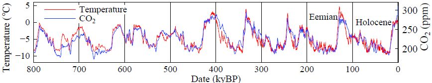
Fig. 2. Antarctic Dome C temperature for past 800 ky from Jouzel et al.(2007) 43 relative to the
mean of the last 10 ky and Dome C CO 2 amount from Luthi et al. (2008). 44
9
This nearly precise agreement is not indicative of the true uncertainty in the GHG forcing, which
IPCC AR6 estimates as 10%, thus about 0.4 W/m 2 . In Supporting Materials, we show that our
CH 4 forcing is larger than that of IPCC AR6, while our MPTG + OTG forcing is smaller than
that of IPCC AR6; these differences approximately offset. The forcing calculation is difficult
because it must account for the complex spectral variability of gaseous absorption and the four-
dimensional variability of water vapor and clouds, but modern computer capability makes more
accurate assessment possible via systematic model intercomparisons. Improved knowledge of
atmospheric radiative properties is needed as humanity works to limit GHGs and otherwise
affect Earth’s energy balance so as to limit undesirable climate change.
The stunning conclusion is that the GHG increase since 1750 now produces a climate forcing
equivalent to that of 2×CO 2 (our formulae yield F e ~ F s = 4.09 W/m 2 for 2021; IPCC’s AR6 F s =
4.14 W/m 2 ). The human-made 2×CO 2 climate forcing imagined by Charney, Tyndall and other
greenhouse giants 1 is no longer imaginary. At this moment, humanity is taking its first steps into
the period of consequences. Earth’s paleoclimate history helps us assess potential outcomes.
Glacial-to-interglacial climate oscillations
Air bubbles in Antarctic ice cores – trapped as snowfall piled up and compressed into ice –
preserve a record of long-lived GHGs for at least the past 800,000 years. Isotopic composition of
the ice provides a measure of temperature change in and near Antarctica. 43 In general, CO 2 , CH 4
and N 2 O were more abundant in interglacial periods than in glacial periods.
Changes of Antarctic temperature and GHGs, especially CO 2 , are highly correlated (Fig. 2). This
does not imply that GHGs were the primal cause of the climate oscillations. Hays, Imbrie and
Shackleton 45 showed that small changes of Earth’s orbit about the Sun and the tilt of Earth’s spin
axis relative to the orbital plane are pacemakers of the ice ages. These orbital changes alter the
seasonal and geographical distribution of insolation, which initiates change of ice sheet size and
GHG amounts. Both of these are mechanisms for glacial-interglacial climate change, but the
reason long-term climate is so sensitive is the further role of ice sheets and GHGs as amplifying
feedbacks. As Earth warms, ice sheets shrink, thus exposing a darker surface that absorbs more
sunlight and warms Earth; this effect works in the opposite sense as Earth cools. Also, as Earth
warms, the ocean and continents release GHGs to the air, which amplifies the warming; as Earth
cools, the ocean and continents take up these gases, which amplifies the cooling. 46
The weak orbital forcings oscillate slowly over tens and hundreds of thousands of years. 47 The
picture of how Earth orbital changes drive millennial climate change was first painted clearly in
the 1920s by Milutin Milankovitch, who built on 19 th century hypotheses of James Croll and
Joseph Adhémar. Paleoclimate changes of ice sheet size and GHG amount in response to global
temperature change are sometimes described as slow feedbacks. 48 They change slowly in the
paleoclimate record, because they are paced by the slowly changing Earth orbital forcing.
However, this does not mean that these feedbacks cannot operate more rapidly in response to a
rapid climate forcing. Indeed, we will conclude that GHG and ice sheet feedbacks partially
respond well before the fast-feedback response to a climate forcing is complete.
Today it is possible to evaluate ECS precisely via comparison of stable climate states before and
after a glacial-to-interglacial climate transition. GHG amounts are known from ice cores and ice
sheet sizes can be inferred from sea level and other geologic data. A warm LGM suggested by
CLIMAP and MARGO 49 data (~3°C cooler than the Holocene) can be firmly rejected, because it
is now certain that their SST data yield a planet out of energy balance by more than 2 W/m 2 , as
discussed above. An energy imbalance of +2 W/m 2 is enough to raise the temperature of the
upper kilometer of the ocean 2.2°C or melt ice to raise sea level 22 m in a century 50 – and 10
times those amounts in a millennium. Such change rates did not occur, so the LGM was more
than 3°C cooler than today. As discussed above, we accept the recent paleo analyses concluding
that the LGM was at least ~6°C cooler than the Holocene.
The Holocene is an unusual interglacial. It began as expected: the maximum glacier melt rate
was at 13.2 kyBP (kiloyears before present) 51 and, after peaking early in the Holocene, GHG
amounts began to decline as in most interglacials. However, several ky later, CO 2 and CH 4 began
to increase, which raised a question of whether humans were beginning to affect GHG amounts.
Ruddiman 52 suggested that CO 2 began to be affected by deforestation 8 ky ago and CH 4 by rice
irrigation 5 ky ago. That issue does not prevent us from using the LGM-Holocene comparison to
estimate ECS, but for the sake of clarity we compare the LGM with both the early and late
Holocene. In addition, we compare the prior glacial maximum (PGM) 53 with the subsequent
interglacial (Eemian, about 130-118 kyBP). Based on a review 54 of Eemian data, we estimate
that the Eemian was about +1°C warmer than the average Holocene temperature. The review
includes a robust estimate of peak Eemian SSTs of +0.5 ± 0.3°C relative to 1870-1889, 55 which
is +0.65 ± 0.3°C relative to our base period 1880-1920 and is consistent with our estimate of
+1°C for land plus ocean Eemian peak warmth.
LGM-Holocene and PGM-Eemian evaluation of ECS
CO 2 , CH 4 and N 2 O amounts in the Holocene, LGM, Eemian and PGM are known accurately
from ice cores, with the exception of N 2 O in the PGM when N 2 O reactions with dust in the ice
core corrupt the data. 56 We take PGM N 2 O as the mean of the smallest reported PGM amount
and the LGM amount. The resulting potential error in the N 2 O forcing is of order 0.01 W/m 2 .
We calculate CO 2 , CH 4 , and N 2 O forcings using Eq. (3) and formulae for each gas in Supporting
Material. We provide 57 GHG amounts and calculated forcings for the periods shown by green
bars in Fig. 3. The period chosen in the Eemian avoids the early spike of CO 2 and temperature to
assure that it is a period with Earth in energy balance. Between the LGM (18-24 kyBP) and late
Holocene (1-5 kyBP), GHG forcing increased 2.5 W/m 2 with 2.0 W/m 2 (80%) from CO 2 .
Between the LGM and early Holocene, GHG forcing increased 2.15 W/m 2 with 80% from CO 2 .
Between the PGM and Eemian, GHG forcing increased 2.3 W/m 2 with 79% from CO 2 .
10
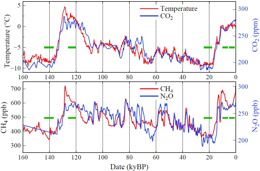
Fig. 3. Antarctic (dome C) temperature (Jouzel et al. 43 ) and multi-ice core GHG amounts (Schilt
et al.). 56 Green bars (1-5, 6-10, 18-24, 120-126, 137-144 kyBP) are periods of calculations.
Earth’s surface changes are the other forcing required to evaluate ECS: (1) change of surface
albedo (reflectivity) and topography due to ice sheets, (2) vegetation change, e.g., interglacial
boreal forests replaced by brighter tundra, and (3) continental shelves exposed by lower sea level
in glacial times. The forcing caused by all three changes can be evaluated at once with a global
climate model. Accurate assessment requires realistic simulation of clouds, which reduce surface
albedo effects. Clouds are the most important and difficult fast feedback (rapid response) in
global climate models. 58 Thus, evaluation of the surface forcing is ideal for PMIP 59
(Paleoclimate Modelling Intercomparison Project) collaboration with CMIP 60 (Coupled Model
Intercomparison Project); a joint study could provide valuable model intercomparisons as well as
assessment of the most important climate characteristic: climate sensitivity.
Aerosols are a final issue to address before estimating climate sensitivity. Human-made aerosols,
including their effect on clouds, are a climate forcing (an imposed perturbation of Earth’s energy
balance). Natural aerosol changes are, like clouds and water vapor, a fast climate feedback.
Indeed, aerosols and clouds form a continuum and distinction becomes arbitrary as humidity
approaches 100 percent. There are many aerosol types, including VOCs (volatile organic
compounds) produced by trees, sea salt produced by wind and waves, black and organic carbon
produced by forest and grass fires, dust produced by wind and drought, and marine biologic
dimethyl sulfide and its secondary aerosol products. All of these vary geographically and in
response to climate change. We cannot accurately specify their properties in prior eras, and there
is no need to do so, because their changes are feedbacks included in the climate response.
Sherwood et al. 28 review studies of LGM ice sheet forcing and settle on –3.2 ± 0.7 W/m 2 , the
same as the IPCC AR4 estimate. 61 However, some GCMs yield efficacies for ice sheet forcings
as low as ~0.75 62 or even ~0.5, 63 i.e., the response to the ice sheet forcing is a fraction of the
11
response to an equal CO 2 forcing. For LGM vegetation, we 7 found a forcing of – 0.9 W/m 2 by
using the Koppen 64 scheme to relate vegetation to local climate. Kohler et al. 65 estimate a
continental shelf forcing of – 0.6 W/m 2 . We estimate the net LGM-Holocene surface forcing as
3-5 W/m 2 , with the wide range due to the uncertain efficacy of the surface forcing. For the time
being – until more accurate assessment of surface forcing is available – let’s use the mean
Holocene GHG forcing of 2.3 W/m 2 , which makes the total LGM-Holocene forcing 5.3-7.3
W/m 2 . Taking the LGM-Holocene warming as 6.1°C 23 and 2×CO 2 forcing as 4 W/m 2 yields ECS
= 3.3-4.6°C for 2×CO 2 . Osman, Tierney et al. LGM cooling of 6.8°C for 23-19 ky BP yields
ECS = 3.7-5.1°C.
PGM-Eemian climate change provides a check. PGM-Eemian GHG forcing was 2.3 W/m 2 . PGM
sea level was ~10 m higher than LGM sea level. 66 The North American ice sheet was smaller
than in the LGM and the Eurasian ice sheet was probably larger. 53 Redistribution of ice mass
between the two major ice sheets has little effect on their combined climate forcing, but less ice
mass by the equivalent of 10 m of sea level reduces the surface forcing by ~0.3 W/m 2 ; see Fig.
S4 in Target CO 2 paper. 67 PGM-Eemian global warming was at least as great as LGM-Holocene
global warming. The PGM was probably slightly warmer than the LGM, as suggested by the
higher PGM sea level and the temperature inferred at Dome C in Antarctica (Fig. 2). However,
temperature at Dronning Maud Land in Antarctica seems to have been cooler in the PGM than in
the LGM. 68 The global Eemian temperature was about 1°C warmer than the Holocene, as
discussed above. In summary, PGM-Eemian warming was several tenths of a degree greater than
the LGM-Holocene warming, while the forcing maintaining Eemian warmth was a few tenths of
a W/m 2 smaller than the Holocene forcing. Thus, while the LGM-Holocene climate change
implies ECS =3.3-5.1°C for 2×CO 2 , the PGM-Eemian implies ECS ~ 4-6°C.
We conclude ECS is at least approximately 4°C and is almost surely in the range 3.5-5.5°C. The
IPCC AR6 conclusion that 3°C is the best estimate for ECS is inconsistent with paleoclimate
data. Our conclusion also applies for transition to warmer climates, as discussed in the Summary
below. Charney’s estimate of 3°C for 2×CO 2 , thus ¾°C per W/m 2 forcing, stood as the canonical
ECS estimate for more than 40 years. Precise data for equilibrium paleo climate states point to a
new canonical ECS: 1°C per W/m 2 forcing. The one major caveat is uncertainty in the glacial
surface climate forcing. A well-designed PMIP/CMIP study could narrow that uncertainty.
High climate sensitivity has implications for climate response time and the amount of warming
in-the-pipeline. Slow climate response – delayed climate response – has policy implications.
12
CLIMATE RESPONSE TIME
Climate response time was surprisingly long in our climate simulations 7 for the 1982 Ewing
Symposium. The e-folding time – the time for surface temperature to reach 63% of its
equilibrium response – was about a century. The only published atmosphere-ocean GCM – that
of Bryan and Manabe 69 – had a response time of 25 years, while several simplified climate
models referenced in our Ewing paper had even faster responses. The longer response time of
our climate model was largely a result of high climate sensitivity – our model had an ECS of 4°C
for 2×CO 2 while the Bryan and Manabe model had an ECS of 2°C.
The physics is straightforward. If the delay were a result of a fixed source of thermal inertia, say
the ocean’s well-mixed upper layer, response time would increase linearly with ECS because
most climate feedbacks come into play in response to temperature change driven by the forcing,
not in direct response to the forcing. Thus, a model with ECS of 4°C takes twice as long to reach
full response as a model with ECS of 2°C, if the mixed layer provides the only heat capacity.
However, while the mixed layer is warming, there is exchange of water with the deeper ocean,
which slows the mixed layer warming. The longer response time with high ECS allows more of
the ocean to come into play. If mixing into the deeper ocean is approximated as diffusive, surface
temperature response time is proportional to the square of climate sensitivity. 70
Slow climate response accentuates need for the “anticipation” that E.E. David, Jr. spoke about. If
ECS is 4°C, more warming is in the pipeline than widely assumed. The greater warming could
eventually make much of the planet inhospitable for humanity and cause the loss of coastal cities
to sea level rise. We will argue that these fates can still be avoided via a reasoned policy
response, but we must understand climate response time to define effective policies.
Temperature response function
In the Bjerknes lecture 71 at the 2008 American Geophysical Union meeting, the first author
(JEH) argued that the ocean in many 72 GCMs has excessive, unrealistic mixing, and he suggested
that GCM modeling groups report and make available the global temperature response function
of their models. The response function is global temperature response to instantaneous doubling
of carbon dioxide (2×CO 2 ) with the model run long enough to approach equilibrium. The
response function characterizes a climate model and allows rapid (Green’s function) estimate of
the global mean surface temperature history in response to any climate forcing:
T G (t) = ʃ [dT G (t)/dt] dt = ʃ λ × R(t) [dF e /dt] dt. (4)
T G is the Green’s function estimate of global temperature at time t, λ (°C per W/m 2 ) the model’s
2×CO 2 equilibrium sensitivity, R the dimensionless temperature response function (% of
equilibrium response), and dF e the forcing change per unit time, dt. The integration over time
begins when Earth is in near energy balance, e.g., in preindustrial time. The response function
yields an accurate estimate of global temperature change for any climate forcing history, with
nearly the same result as that of the global GCM that produced the response function (see Chart
15 of the Bjerknes presentation). 71 This approximation is expected to be good for any forcing
unless and until the forcing causes a fundamental reorganization of the global ocean circulation.
13

Fig. 4. (a) Global mean surface temperature response to instant CO 2 doubling and (b) normalized
response function (percent of final change). Thick lines in Figs. 4 and 5 are smoothed 73 results.
Ocean mixing is addressed by comparison of two versions of the GISS GCM: GISS (2014) 74 and
GISS (2020). 35 Both models 75 are described by Kelley et al. (2020). 34 Ocean mixing is markedly
improved in GISS (2020) by use of a high-order advection scheme, 76 finer upper-ocean vertical
resolution (40 layers), updated mesoscale eddy parameterization, and correction of errors in the
ocean modeling code. 34 The GISS (2020) model has improved internal variability, including the
Madden-Julian Oscillation (MJO), El Nino Southern Oscillation (ENSO) and Pacific Decadal
Oscillation (PDO), although the spectral signature of the ENSO-like variability is unrealistic and
its amplitude is excessive, as shown by the magnitude of oscillations in Fig. 4a. Ocean mixing in
GISS (2020) may still be a bit excessive in the North Atlantic, where the model’s simulated
penetration of CFCs is greater than observed. 77
Despite reduced ocean mixing, the response time of surface temperature in the GISS (2020)
model is no faster than the GISS(2014) model (Fig. 4b): it takes 100 years to reach within 1/e of
the equilibrium response. Slow response is partly explained by the larger ECS of the GISS
(2020) model, which is 3.5°C versus 2.7°C for the GISS (2014) model, but something more is
going on in the newer model, as exposed by the response function of Earth’s energy imbalance.
Earth’s energy imbalance
When Earth’s climate is perturbed by a forcing, the resulting Earth energy imbalance (EEI)
drives warming or cooling that tends to restore balance. Increasing GHGs and decreasing
aerosols at present cause a positive EEI – more energy coming in than going out – by about +1
W/m 2 averaged over several years. 78 Highest absolute accuracy of EEI is obtained by tracking
ocean warming – the primary repository for excess energy – and by adding the heat stored in
warming of continents and the heat used in net melting of ice. 78 Heat storage in air adds a small,
almost negligible, amount. Observations of radiation balance from Earth-orbiting satellites by
themselves cannot measure EEI to the needed accuracy, but, when calibrated with the in situ
data, satellite Earth radiation budget observations provide invaluable EEI data on finer temporal
and spatial scales than the in situ data. 79
14

Fig. 5. (a) Earth’s energy imbalance (EEI) for 2×CO 2 , and (b) EEI normalized response function.
After a step-function forcing is imposed, EEI and global surface temperature must each approach
a new equilibrium, but EEI does so more rapidly, especially for the GISS (2020) model (Fig. 5).
EEI in the GISS (2020) model needs only a decade to reach within 1/e of full response (Fig. 5b),
while global surface temperature requires a century (Fig. 4b). Rapid decline of EEI – to half the
forcing within 5 years (Fig. 5a) – has practical implications, if it is realistic. First, EEI defines the
rate that heat is pumped into the ocean, so if EEI is reduced, ocean surface temperature response
time increases. Second, rapid EEI decline – if it is realistic – implies that the assumption that
global warming and pumping of heat into the ocean can be stopped if humanity reduces climate
forcing by an amount equal to EEI may be wrong. Instead, the required reduction of forcing is
probably larger than EEI. In any scenario to stabilize climate, the difficulty in finding additional
reduction in climate forcing of even a few tenths of a W/m 2 is substantial. 54 Calculations that can
help quantify this issue are discussed in Supporting Material.
What is the physics behind the fast response of EEI? The 2×CO 2 forcing and initial EEI are both
nominally 4 W/m 2 . In the GISS (2014) model, the decline of EEI averaged over the first year is
0.5 W/m 2 (Fig. 5a), a moderate decline that might be largely caused by warming continents and
increased heat radiation to space. In contrast, EEI declines 1.3 W/m 2 in the GISS (2020) model
(Fig. 5a). Such a huge, immediate decline of EEI implies existence of an ultrafast climate
feedback. Climate feedbacks are the heart of climate change and warrant discussion.
Slow, fast and ultrafast feedbacks
Charney et al. 4 described climate feedbacks without discussing time scales. At the 1982 Ewing
Symposium, water vapor, clouds and sea ice were described as “fast” feedbacks 7 presumed to
change promptly in response to global temperature change, as opposed to “slow” feedbacks or
specified boundary conditions such as ice sheet size, vegetation cover, and atmospheric CO 2
amount, although it was noted that some specified boundary conditions, e.g., vegetation, in
reality may be capable of relatively rapid change. 7
Large response of EEI in one year (Fig. 5a) implies a third feedback time scale: ultrafast.
Ultrafast feedbacks are not a new concept. When atmospheric CO 2 is doubled, the added infrared
15
opacity causes the stratosphere to cool. Instantaneous EEI upon CO 2 doubling is only F i = +2.5
W/m 2 , but stratospheric cooling quickly increases EEI to +4 W/m 2 . 80 This quick adjustment led
to the choice of adjusted forcing, F a , as superior to F i as a measure of climate forcing.
Physics behind ultrafast change in the GISS model likely involves cloud change. Indeed, Kamae
et al. 81 review rapid cloud adjustments separate from surface temperature-mediated changes.
Clouds respond to radiative forcing, e.g., via effects on cloud particle phase, cloud cover, cloud
albedo and precipitation. 82 The GISS (2020) model alters glaciation in stratiform mixed-phase
clouds, which increases the amount of supercooled water in stratus clouds, especially over the
Southern Ocean [Fig. 1 in GISS (2020) GCM description 34 ]. The portion of supercooled cloud
water drops changes from too little in GISS (2014) to too much in GISS (2020). Although
neither model realistically simulates stratocumulus clouds – which are important for accurate
simulation of Earth’s albedo and climate sensitivity – that modeling deficiency does not affect
our assessment of climate sensitivity and it does not prevent use of the two GISS models to help
expose real-world physics affecting climate sensitivity and climate response times.
Cloud modeling is now a focus in GCM development. Several models in CMIP6 comparisons
find high ECS. 82 It would be informative if the models defined their temperature and EEI
response functions (Figs. 4 and 5). Failing that, model runs of even a decade could define the
most crucial portion of Figs. 4a and 5a. In addition, if many short (e.g., 2-year) 2×CO 2 climate
simulations were made with each run beginning at a different point in the model’s control run,
ultrafast feedbacks including cloud changes could be defined to an arbitrary accuracy by
averaging the responses and subtracting the same years in the control run. As noted in our
Supporting Material, definition of response functions for just a few forcings – say CO 2 , aerosols
and solar irradiance – would help assess the physical mechanisms causing ultrafast feedbacks
and the physics behind high climate sensitivity.
Zhu et al. 83 recently used the LGM climate to constrain the microphysics and ice nucleation
cloud parameterization in the Community Earth System Model CESM2. The paleo constraint
reduced the ECS of the model from >5°C to 4°C for 2×CO 2 . This independent study with a
model including cloud microphysics is consistent with our inferences and could be a vehicle to
evaluate EEI response with more realistic cloud physics. If the EEI response is much faster than
the temperature response, it implies that the climate forcing reduction required to stabilize
climate is greater than measured EEI, as discussed in Supporting Material.
The ultrafast response of EEI in the GISS (2020) model also exists, although much smaller, in
the GISS (2014) model, as shown in our Supporting Material. The need for further study of
ultrafast feedbacks and the wide range of climate sensitivities among current GCMs does not
alter the high ECS that we infer from paleoclimate data, as that inference has little dependence
on GCMs. The main role of GCMs in the paleoclimate analyses is to define seasonal and
geographical climate patterns, which allows more accurate assessment of global temperature
change from limited paleo data samples. 23,24,26
Understanding clouds requires understanding aerosols, which are involved in cloud feedbacks.
Human-caused aerosol changes are also a major driver of climate change.
16
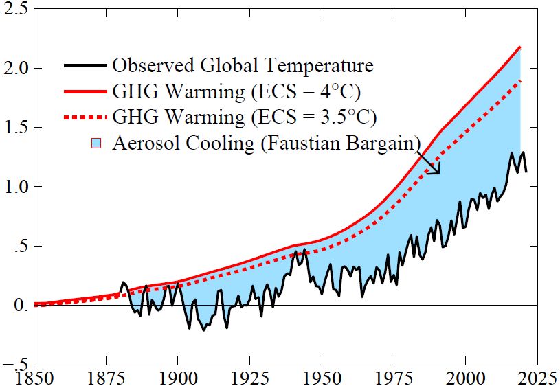
Fig. 6. Observed global mean surface temperature (black line) and expected warming from
observed GHG changes with two alternative choices for ECS. The difference (blue area) is an
estimate of the cooling effect of the (unmeasured) aerosol forcing. The temperature peak in the
World War II era is in part an artifact of inhomogeneous ocean data during that period. 54
AEROSOLS
ECS near 4°C implies that expected warming for today’s GHGs far exceeds observed warming.
Expected GHG warming (Fig. 6) is calculated using equation (4) with the response function (Fig.
4b). 84 For ECS = 4°C, the expected GHG warming today (2.2°C) exceeds observed warming by
about 1°C. If ECS is 3.5°C, the gap is about 0.7°C. The indicated expected warming does not
include warming by slow feedbacks except for a small contribution in observed GHG amounts;
potential further warming by slow feedbacks is discussed quantitatively below.
Human-made aerosols are the likely source of cooling that has partially offset GHG warming.
An alternative source of cooling is human-made increase of Earth’s surface albedo, which occurs
via deforestation, agriculture, road-building, and other human developments, partially offset by
decreased albedo due to deposition of soot on snow and ice surfaces. IPCC 13 (Chapter 7, Table
7.8) estimates the net forcing due to surface albedo change as –0.12 ± 0.1 W/m 2 , which is an
order of magnitude smaller than their estimated aerosol forcing. Thus, in our empirical
evaluation of human-made cooling, we associate almost the entire cooling with aerosols.
Aerosol cooling is described as a Faustian bargain. 85 Payment comes due as we reduce pollution
from shipping, vehicles, industry, and power plants, which we must do because ambient air
pollution causes millions of deaths per year, with particulates most responsible. 86
Aerosol climate forcing is difficult to measure because it occurs mainly via small induced cloud
changes. 13 The absence of significant global warming over the period 1850-1920 (Fig. SPM.1 of
the IPCC AR6 WG1 report) is a clue for the scale of aerosol forcing. GHG forcing increased
+0.54 W/m 2 in 1850-1920, which causes an expected warming ~0.3°C by 1920, based on the
climate response function with 3.5°C ECS (Fig. 4). Natural forcings – solar irradiance and
volcanic aerosols – could contribute to lack of warming, but we are unaware of a persuasive case
17

Fig. 7. Global mean surface temperature (left scale) and climate forcings (right). Scale factor
between temperature and forcings is 2.4°C per W/m 2 (see text). Antarctic (Vostok) temperature
change based on water isotopes 87,88 is multiplied by 0.75. Time scale is expanded post 1750.
Modern temperature is NASA GISS analysis. 89,90 Zero point for GHG forcing is the mean for
10-8 ky BP, a period expected to precede significant human effects. GHG + IPCC aerosol
forcing is indistinguishable from IPCC 13 all-anthropogenic forcing (Supporting Material).
for the required downward trends of those forcings. Aerosols from increasing industrialization
prior to most environmental protection laws are a more likely offset to GHG warming.
Paleoclimate evidence related to human-caused aerosols
Paleoclimate data provide ways to assess aerosol climate forcing. Natural paleo aerosol changes
are fast feedbacks, as discussed above, but human-caused aerosols are a forcing – an imposed
perturbation of Earth’s energy balance. We will examine the continuity of modern climate data
with the paleoclimate record to show the magnitude of warming in the pipeline, if today’s level
of GHGs – or a greater amount – long persists. Then we use the relative stability of Holocene
global temperature to extract evidence that human-made aerosols were a significant climate
forcing during the latter part of the preindustrial Holocene.
In the paper Target CO 2 67 the scale factor between equilibrium global temperature change and
GHG forcing is 1.5°C per W/m 2 of GHG forcing based on an assumed ECS of 3°C for 2×CO 2
(0.75°C per W/m 2 ) and an assumption that GHG and ice sheets contributed about equally to the
glacial-interglacial climate forcing (each 3 W/m 2 ). Our present assessment has ECS of 4°C (1°C
per W/m 2 ) and more precise LGM-to-Holocene GHG forcing (2.5 W/m 2 ) and ice sheet forcing
(3.5 W/m 2 ). Thus, the improved ΔT to F GHG scale factor in Fig. 7 is (F GHG + F Ice )/ F GHG × 1°C per
W/m 2 = 2.4°C per W/m 2 of GHG forcing. Temperature change in the paleo portion of Fig. 7 is
the full observed change, which includes slow feedbacks. Modern temperature (purple curve) has
not had time for the ocean to warm fully or for slow feedbacks to come fully into play.
Paleo GHG forcing in Fig. 7 is the first three terms in Eq. 2 with adjusted forcings for CO 2 , CH 4
and N 2 O from formulae in Supporting Material. The GHG forcings are a fit to radiative transfer
calculations in a GCM 31 and agree well with the net IPCC GHG forcing, as shown above. Fig. 7
18
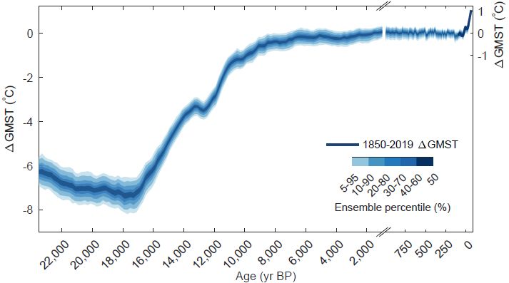
Fig. 8. Global mean surface temperature change over the past 24 ky, reproduced from Fig. 2 of
Osman et al. 24 including Last Millennium reanalysis of Tardif et al. 91
also shows the GHG plus aerosol forcing using IPCC’s estimated aerosol forcing history. There
are gaps in the Vostok N 2 O record prior to 132 ky BP, so we approximate the earlier N 2 O forcing
by increasing the CO 2 + CH 4 forcing by 12 percent. Good accuracy of this approximation is
shown in Supporting Material for the past 132 ky, when N 2 O data are available.
Paleo GHG climate forcing and Antarctic temperature change are nearly congruent (Fig. 7). A
free parameter in Fig. 7 is the factor by which the Vostok temperature change is multiplied to
obtain approximate congruence with the climate forcing. With the climate forcings and climate
sensitivity assumed in Target CO 2 , close congruence of forcing and temperature was achieved if
Vostok temperature change was multiplied by 0.5, i.e., Southern Hemisphere polar amplification
of temperature was a factor of two. With GHG forcing of 2.5 W/m 2 and ECS of 1°C per W/m 2 ,
the factor by which Vostok temperature must be multiplied to achieve close congruence of
temperature and forcing is 0.75 (Fig. 7). Reduced Southern Hemisphere polar amplification is
consistent with recent estimates of LGM-Holocene global temperature change. 23,24,26
Target CO 2 and Fig. 7 use the Vostok temperature derived from water isotopes. 87,88 Recent
analysis 92 of LGM Antarctic cooling based on borehole thermometry and firn properties reveal
that glacial cooling at the ice sheet surface is less than suggested by water isotopes, implying that
the scale factor between Vostok and global temperature may be different from the value (0.75) in
Fig. 7. Neither this specific scale factor for Vostok (where the temperature depends on changing
ice surface height and other local factors) nor ice age polar amplification in general are important
for our present paper. Here we only want to explain clearly the contents of Fig. 7.
A stunning result in Fig. 7 is that equilibrium global warming for today’s GHG level is 10°C.
Aerosols, at their maximum level in the early 21 st century, reduce equilibrium warming to 7°C,
but the aerosol amount is in decline The paleo temperature changes occurred over millennia, on
the time scale of the climate forcing. Today’s GHG forcing is rising faster than any known paleo
case. In a following paper 93 we will use paleoclimate data, climate modeling and modern
observations to assert that a large ice sheet response and several meters of sea level rise are likely
on the century time scale in response to continued extraordinary human-made climate forcing.
19

Fig. 9. GHG climate forcing in past 20 ky with vertical scale expanded for the past 10 ky on the
right. GHG amounts are from Schilt et al. 56 and formulae for forcing are in Supporting Material.
We focus here on the two forcings – human-caused changes of GHGs and aerosols – that are the
dominant causes of ongoing climate change. Volcanic and solar irradiance forcings have notable
short-term variation, but no significant long-term trend. Other human-made forcings estimated
by IPCC have little net effect on total forcing history (see Supporting Material).
Several proxy-based analyses (e.g.) 94,95 found global cooling in the second half of the Holocene,
but a recent analysis 24 that uses GCMs to overcome spatial and temporal biases in proxy data
finds a rising global temperature in the first half of the Holocene followed by nearly constant
global temperature in the last 6000 years until the past few centuries (Fig. 8, extracted from Fig.
2 of Osman et al. 24 ). The deep ocean, tropical sea surface, and Antarctica all had stable
temperature in the last 6000 years (Fig. S6 of Target CO 2 ). 67
The final 6000 years of the Holocene are unusual. GHG forcing (Fig. 9) increased by 0.5 W/m 2 ,
yet global temperature was stable, if not declining. Even the Osman et al. 24 analysis (Fig. 8),
which shows Holocene warming over the last 9000 years, has no warming in the last 6000 years.
Six thousand years is sufficient time for slow feedbacks to operate, as well as fast feedbacks.
Global warming of about 1°C would be expected, based on climate sensitivity implied by Fig. 7.
How can we interpret the absence of warming? Was another climate forcing at work?
Did humanity significantly affect preindustrial climate?
Ruddiman hypothesized 52 that humanity began to influence climate with the advent of land-
clearing and agriculture. In a review 96 of his hypothesis, Ruddiman places the beginning of
significant deforestation at 6500 yr BP and rice irrigation at 5000 yr BP, causing respective
increases of atmospheric CO 2 and CH 4 . In his analysis, Ruddiman seeks human-made sources of
CO 2 and CH 4 of sufficient magnitude to compensate for large declines of those gases in the latter
parts of prior interglacial periods. While we support Ruddiman’s assertion that humans began to
affect climate prior to the industrial revolution, we note that such large sources are unnecessary
to account for Holocene GHG levels. Our principal interest is in preindustrial aerosols, but first
we comment on why Ruddiman’s thesis is more viable than it may have seemed.
20

Fig. 10. Sea level since the last glacial period relative to present. Credit: Robert Rohde 97
GHG decreases during a typical interglacial period are slow feedbacks that occur in concert with
global cooling. However, global cooling did not occur in the past 6000 years, so the feedbacks
did not occur. A principal mechanism in glacial-interglacial swings of atmospheric CO 2 and
global temperature (Fig. 2) is the net rate of uptake of carbon by the deep ocean. Carbon
sequestration in the deep ocean increases if ocean overturning slows because the rate of carbon
return to the atmosphere is reduced. Maximum insolation at 60°S was in late-spring (mid-
November) 6000 years ago; since then, the date of maximum insolation at 60°S slowly advanced
through the year, recently passing mid-summer (Fig. 26b of Hansen et al. 14 ). Maximum
insolation from late-spring through mid-summer is optimum for direct warming of the Southern
Ocean and for promoting early warm-season ice melt, which reduces surface albedo and
magnifies regional warming. 48 Thus, Earth orbital parameters were optimum for keeping the
Southern Ocean warm as needed to maintain a strong overturning ocean circulation.
GHG forcing decreased 0.2 W/m 2 between 10 and 6 ky BP, but the decrease was exceeded by a
forcing due to shrinkage of ice sheets. Sea level 10 ky ago was 40 m below today (Fig. 10); loss
of that ice causes a climate forcing of just over +1 W/m 2 , as shown in Supporting Material of the
Target CO 2 paper. 67 Error! Bookmark not defined. The net forcing was enough to produce the
global warming of less than or about 1°C deduced from paleo data for the period 10-6 ky BP
(Fig. 8). The mystery is the past 6000 years, when sea level and thus ice sheet volume were
static. The 0.5 W/m 2 rise of GHG forcing over 6000 years must have been counteracted by a
comparable negative forcing to yield the near constant global temperature deduced by Osman et
al. 24 An even larger negative forcing is required, if there was global cooling in the past 6000
years.
Hansen et al. 48 suggested that human-made aerosol cooling offset or exceeded GHG warming in
the past 6000 years. Growth of population, agriculture and land clearance 96 produced aerosols as
well as CO 2 . Wood was the principal fuel for cooking and heating. As today, the largest aerosol
forcing would be via effects on cloud cover and cloud brightness. This aerosol indirect effect
21
tends to saturate as aerosol amount increases, so aerosol effectiveness per aerosol amount was
greatest as civilization developed. Thus, it is unsurprising that human-made global aerosol

Fig. 11. (a) Estimated greenhouse gas and aerosol climate forcings relative to 1750 values. (b) Aerosol
climate forcing as percent of GHG forcing that it offsets. Aerosol and GHG forcings for dark blue area
are relative to 1750 values. Light blue area is added when the GHG and aerosol forcings are defined
relative to their values 6000 years ago, with GHG and aerosol forcings both reaching 0.5 W/m 2 by 1750.
forcing approximately offset human-made CO 2 forcing, as required to explain the absence of
global warming in the past 6000 years of preindustrial climate.
Hemispheric differences provide a consistency check. GHG (mainly CO 2 ) forcing is global,
while the aerosol forcing was mainly in the Northern Hemisphere. Global offset of the two
forcings implies a net negative forcing in the Northern Hemisphere and positive forcing in the
Southern Hemisphere. Therefore, human-made aerosols were likely a contributor to observed
Northern Hemisphere cooling, which occurred on at least a regional scale, while GHG warming
in the Southern Hemisphere helped orbital forcing keep the Southern Ocean warm.
Industrial era aerosols
Scientific advances often face early resistance from other scientists. 98 Examples are the snowball
Earth hypothesis 99 and the role of an asteroid impact on extinction of non-avian dinosaurs, 100
which initially were highly controversial but are now more widely accepted. Ruddiman’s
hypothesis, right or wrong, is still controversial. Thus, we minimize this issue by showing
aerosol effects with and without preindustrial human-made aerosols.
Global aerosol properties have not been monitored with the detail and accuracy needed to define
the aerosol climate forcing, 101 but IPCC 13 estimates the aerosol forcing (Fig. 11a) based on
assumed aerosol precursor emissions – mainly related to fossil fuel use – and aerosol models that
are tested against a range of observations in recent decades. The task is difficult because of the
multitude of aerosol types and the complex effects of aerosols on clouds. Uncertainty in aerosol
forcing is at least 50 percent of the estimate in Fig. 11a 13 and probably is constrained more by
observed global temperature change than by measurements of aerosols or precursor gases.
Using IPCC’s best estimate aerosol forcing history (Fig. 11a) and the accurately known GHG
history, we calculate the percent of GHG climate forcing offset by aerosol cooling – the dark
blue area in Fig. 11b, which is simply the ratio of aerosol and GHG forcings. However, if
human-made aerosol forcing was – 0.5 W/m 2 by 1750, offsetting the known +0.5 W/m 2 GHG
forcing in 1750 (regardless of whether or not the GHG forcing was human-made), that aerosol
forcing should be included in the total aerosol forcing and offset a 1750 GHG forcing of 0.5
W/m 2 (Fig. 9). This 1750 aerosol forcing – largely cloud effects of aerosols from land use,
22
human-caused fires, and burning of biomass – is assumed to continue until today. The picture of
the aerosol role in climate change, shown by both shades of blue in Fig. 11b, thus changes when
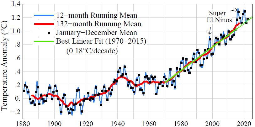
Fig. 12. Observed global surface temperature change relative to 1880-1920 based on GISS
analysis. 89,90 Data for 2022 is January-October mean. Monthly updates are available. 102
the full effect of aerosols from land-use and human-caused fires is included. Aerosol offset of
GHG warming was dominant until about 1970. The relative decline of aerosol forcing after 1970
(Fig. 11b) reflects the effect of clean air laws in parts of the world.
Fig. 11b, with and without the (light blue) preindustrial aerosols, encapsulates two alternative
views of the historical role of human-caused aerosols. IPCC’s aerosol history, with aerosol
forcing gradually becoming important relative to GHG forcing, derives from aerosol simulations
driven mainly by fossil fuel emissions. In the alternative view, civilization always produced
aerosols as well as GHGs. Organized societies and rapid population growth began on coasts as
stabilizing sea level increased coastal margin biologic productivity 103 and inland as agriculture
developed. Wood was the main fuel; it would be surprising if the growing human population did
not produce aerosols that affected clouds of a prior virgin atmosphere. Aerosols travel great
distances, as shown by the presence of Asian aerosols in the United States and by satellite
tracking of fire-produced aerosols. Small aerosol amounts in otherwise pristine marine air can
produce a significant climate forcing. In our view, humans likely contributed to both rising GHG
and aerosol climate forcings in the past 6000 years. No persuasive alternative explanation has
been proffered for the absence of global warming in that period of increasing GHG amounts.
At face value, the steep decline in the aerosol offset of GHG forcing beginning in the early 1970s
(Fig. 11b) – a result of stabilization of global aerosol forcing (Fig. 11a) – is a triumph of aerosol
modeling, providing a partial explanation for the steep global temperature rise that began at that
time (Fig. 12). However, we must bear in mind that the temperature record was known when the
aerosol scenarios were developed. It is not a case of prediction and observational confirmation.
23
One implication of our alternative view of aerosol forcing history is that the human-caused
negative aerosol climate forcing is 0.5 W/m 2 larger than obtained from models that deal with
aerosol change only in the past century or two. Thus, the Faustian payment that will eventually
come due is probably larger than usually assumed, as discussed below.
Global temperature and EEI constraints on aerosols and climate models
Global warming in the past 100 years (Fig. 12) is commonly used to estimate climate sensitivity,
but by itself it is ill-suited for that purpose. Global warming does not yield a unique climate
sensitivity because the warming depends on three major unknowns with only two fundamental
constraints. 15 Unknowns are: ECS, net climate forcing (uncertain because aerosol forcing is
unmeasured), and ocean mixing (uncertain based on evidence that many ocean models are too
diffusive). Constraints are observed global temperature change (Fig. 12) and EEI. 78 Accurate
knowledge of EEI began with the Argo float program, 104 which initiated well-calibrated
measurements of ocean heat content globally in the first decade of the 21 st century.
In an analysis 105 using early Argo data, we reduced unknowns to two by assuming ECS = 3°C.
From EEI ~ 0.58 W/m 2 for the 2006-2010 solar minimum, we inferred a solar cycle mean EEI ~
0.75 W/m 2 . Our aerosol forcing versus time was from aerosol modeling of Koch 106 that
incorporated changing technology factors defined by Novakov. 107 We solved for aerosol forcing
in 2010, obtaining –1.63 ± 0.3 W/m 2 relative to 1880 – in the range estimated in the radiative
forcing chapter of IPCC reports, but more negative than aerosol forcing used in most GCMs in
CMIP and IPCC reports. Our interpretation – in agreement with Knutti 108 – was that most
climate models compensate for excessive ocean mixing (which reduces surface warming) by
using aerosol forcing less negative than the real world to achieve realistic global warming.
With ECS uncertain, we are back to an underdetermined system. Moreover, response functions
for the GISS GCMs (Figs. 4 and 5) imply that climate response depends on more than ECS and
ocean mixing; atmospheric processes also affect climate response time. We infer – for want of a
likely alternative – that cloud changes are probably involved in the ultrafast feedbacks. Thus, a
comprehensive analysis must include analysis of the role of cloud feedbacks in global climate
change. A first step is to assess the mechanisms in ultrafast feedbacks, which can be done via
many short (~2 year) GCM runs for 2×CO 2 , as described above. If CMIP included such short
simulations, it may identify observable feedbacks that produce high ECS in several GCMs. 82 A
second step is to define response functions individually for CO 2 , aerosols and solar irradiance.
Aerosols, located mainly beneath clouds, may have a different response function than GHGs.
The solar variability response is needed because the period with accurate EEI data is limited;
solar change is a significant portion of the forcing change in that period.
Such an analysis would require many GCM runs and is beyond the scope of this paper. Instead,
for the purpose of estimating today’s aerosol climate forcing, we make the usual assumption that
effective forcings defined by a primitive GCM 31 allow all forcings to be treated as equivalent and
thus we use of a single response function in Eq. (4). This assumption is called into question by
the indirect evidence that cloud feedbacks may be more complex and have a larger effect than in
early GCMs, yet we may be able to draw some general conclusions with appropriate caveats.
Aerosol climate forcing and future warming estimates
24
Many combinations of climate sensitivity and aerosol forcing are consistent with observed global
warming. 15 The response function for the GISS (2014) model yields a result (Fig. 13) typical of
models in CMIP and IPCC reports: AR6 aerosol forcing yields good agreement with observed
warming in the last half century – the period when human-made climate forcing overwhelms

Fig. 13. Global temperature change T G due to aerosols + GHGs calculated with Green’s function
Eq (4) using GISS (2014) and (2020) response functions (Fig. 4). Observed temperature is the
NASA GISS analysis. 89,90 Base period: 1951-1980 for observations and model.
natural forcings, unforced climate variability, and flaws in observed warming due to inadequate
data. However, agreement with observed temperature also can be achieved by climate models
with high ECS. The GISS (2020) model, with ECS = 3.5°C, yields greater warming than
observed if IPCC aerosol forcing is used (Fig. 13), but less warming than observed for the
aerosol scenario inferred in our 2011 EEI study. 105 This latter aerosol scenario yields close
agreement with observed warming if ECS ~ 4°C (green curve in Fig. 13). 109 Agreement also can
likely be achieved with a still higher ECS by use of a larger (more negative) aerosol forcing.
IPCC AR6 WG1 best estimate aerosol forcing (Table AIII.3) 13 is near maximum (negative) value
by 1975, then nearly constant until the 21 st century, when it rises to –1.09 W/m 2 in 2019 (Fig.
14). This AR6 aerosol forcing is in the upper (less negative) portion of the range estimated in the
radiative forcing chapter of AR6. 110 In contrast, some aerosol models, including those of Koch 106
and Bauer (Fig. 14), yield substantial growth of aerosol forcing after 1975.
25
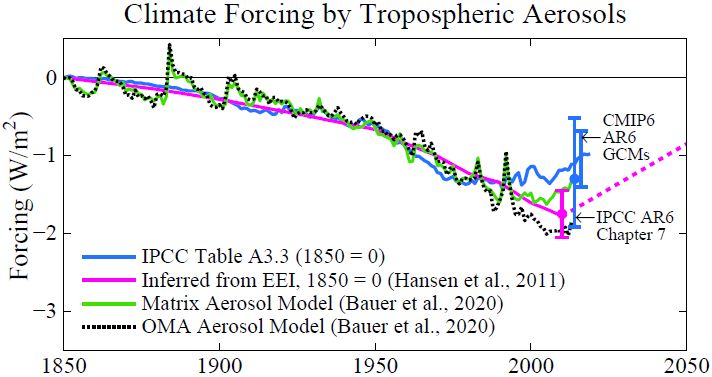
The issue we raise is the magnitude of aerosol forcing. Aerosol forcing is unmeasured and hard
to model because it involves complex aerosol effects on clouds. The result is wide latitude in the
aerosol forcing used in climate simulations. Two GCM problems cause a tendency to minimize
aerosol forcing: (1) excessive mixing of heat into the deep ocean, and (2) a too-small ECS, likely
due to GCM failure to fully capture cloud feedbacks. An analysis based on observed EEI and
global temperature, largely independent of GCMs, concluded 105 that aerosol forcing was about –
1.6 W/m 2 in 2010 relative to 1880. Our present finding of ECS ~ 4°C favors a slightly larger
aerosol forcing (Fig. 13) for consistency with observed global warming. 112 We conclude that the
peak human-made aerosol forcing was likely in the (negative) range 1.5-2 W/m 2 relative to
preindustrial and more negative relative to a pristine (pre-human) atmosphere.
Declining aerosol amount implies acceleration of global warming above the 1970-2010 rate
(0.18°C per decade). Just as 1970 was a hinge point for global warming (Fig. 12), so 2010 is
another hinge point as it marks transition to declining aerosols from China (a decline not
captured well in most CMIP6 models 113 ), where emissions of SO 2 (a principal precursor of
aerosols) declined 70 percent between 2006 and 2017, 114 and strengthening of regional and
global regulations on ship emissions in 2015 and 2020 by the International Maritime
Organization (IMO). 115 A review 116 of aerosol forcing estimates for 2000-2019 found a
consensus that aerosol forcing decreased (became less negative), but the decrease among the
estimates ranged from about 0.1 W/m 2 to about 0.3 W/m 2 for the 20-year period. Uncertainties in
each case are substantial, but together they make a persuasive case that the change of aerosol
forcing in that period is of the opposite sign from that in the 20 th century, i.e., aerosol change no
longer partly offsets growth of GHG climate forcing, rather it adds to the GHG forcing growth.
Expectation of continued decline in aerosol amount is based in part on growing concern about
health effects of aerosol pollution that causes millions of deaths per year 86 and global trends
toward renewable energy, nuclear power, and replacement of coal by gas. Reduction of human-
made aerosols by half between 2010 and 2050 would contribute a climate forcing about +0.2
W/m 2 per decade. Although an aerosol reduction that rapid is uncertain, we expect some
reduction and a forcing increase of at least +0.1 W/m 2 per decade for the reasons given here.
26
Average GHG climate forcing increase since 1970 is about 0.45 W/m 2 per decade, but about 0.5
W/m 2 in the past decade (Fig. 15). This graph includes all well-mixed GHGs and changes of O 3
and stratospheric H 2 O associated with CH 4 change. It thus misses only about half of the O 3
change, which is estimated to cause a forcing of about 0.2 W/m 2 over 1750-2021, about 5% of
the total GHG forcing (see Supporting Material). GHG climate forcing growth has continued
unabated since the 1997 Kyoto Protocol and subsequent agreements of the Conference of the
Parties (COP) meetings, such as the Paris Agreement of 2015, and the growth rate has even
increased. For reasons given in the Discussion section below, we expect a similar growth rate to
continue for the next few decades, at least as long as polices are based on goals and targets.
During 1970-2010 the drive for global warming increased ~0.3 W/m 2 per decade (+0.45 W/m 2
for GHGs, –0.15 W/m 2 for aerosols). Going forward from 2010 for a few decades, we expect this
drive to be at least 0.5-0.6 W/m 2 per decade, for reasons given above. Global temperature
responds reliably to climate forcing on decadal time scales, with about 50% of the response in
the first decade, with about 15% more in the next 100 years (Fig. 4b). Thus, the rate of global
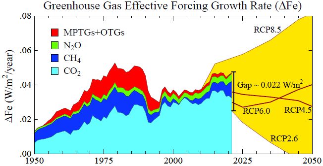
Fig. 15. Update 41 of annual growth of climate forcing by GHGs, including part of O 3 forcing via
the efficacy of CH 4 forcing (cf. Supporting Material). MPTG and OTG are Montreal Protocol
and Other Trace Gases. RCP2.6 is a scenario designed to keep global warming below 2°C.
temperature change in 2010-2040 should be nearly proportional to the multi-decadal growth rate
of the climate forcing. Therefore, we estimate that the global warming rate in 2010-2040 will be
at least 50% greater than in 1970-2010, i.e., at least 0.27°C per decade.
Interpretation of past climate change and prediction of the future could be more precise if aerosol
climate forcing were monitored. Aerosol monitoring could be analogous to the method used for
GHGs. The GHG forcing is obtained by measuring GHG changes accurately and making a
radiative transfer calculation with a realistic global distribution of clouds. A similar approach for
aerosols requires global monitoring of changes of aerosol and cloud particle microphysics with
precision adequate to define their climate forcing. 117,118 In the absence of such Keeling-like
global monitoring, progress has been made via limited satellite measurements of aerosol and
cloud properties, field studies, and aerosol and cloud modeling. These data provide an estimate
of the small direct aerosol forcing in cloud-free regions. The indirect forcing caused by aerosol-
induced cloud changes must be extracted from natural (unforced) cloud variability and cloud
27
changes caused by ongoing global warming. In the absence of precise global monitoring of
aerosol and cloud particle microphysics, progress has relied heavily on modeling of aerosol-
cloud physics and testing results against specific observations.
The great inadvertent aerosol experiment
Sulfate aerosols are a cloud condensation nuclei (CCN), so ship emissions result in a larger
number of smaller cloud particles, affecting cloud albedo and cloud lifetime. 119 Ships provide a
large percentage of sulfates in the North Pacific and North Atlantic regions (Fig. 16). Ship-tracks
(cloud trails) produced by aerosol CCN are apparent, but it has been suggested that cooling by
these clouds is overestimated because of cloud liquid water adjustments. 120 On the other hand,
Manshausen et al. 121 present evidence that liquid water path (LWP) effects are mis-estimated,
including regions without visible ship-tracks; they estimate a LWP forcing – 0.76 ± 0.27 W/m 2 ,
in stark contrast with the IPCC estimate of + 0.2 ± 0.2 W/m 2 . Wall et al. 122 use satellite
observations to quantify relationships between sulfates and low-level clouds; with help of the
“opportunistic experiment” provided by decrease of air pollution downwind of eastern North
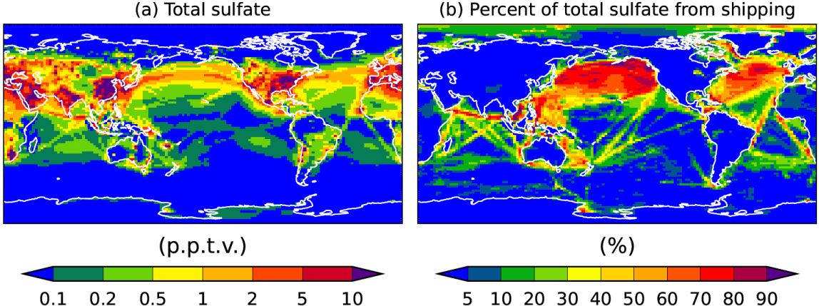
Fig. 16. Total sulfate (parts per trillion by volume) and percentage of total sulfate provided by
shipping in simulations of Jin et al. 123 prior to IMO regulations on sulfur content of fuels.
America, they infer a sulfate indirect aerosol forcing of – 1.11 ± 0.43 W/m 2 over the global
ocean, consistent with our inference of a large (negative) total aerosol forcing.
IMO emission regulations provide a great opportunity for insight into aerosol climate forcing.
Sulfur content of fuels was limited to 1% in 2010 near the coasts of North America and in the
North Sea, Baltic Sea and English Channel, and further restricted there to 0.1% in 2015. 115 In
2020 a limit of 0.5% was imposed worldwide. The 1% limit did not have a noticeable effect on
ship-tracks, but a striking reduction of ship-tracks was found after the 2015 IMO regulations,
especially in the regions near land where emissions were specifically limited. 124 Following the
additional 2020 regulations, 125 global ship-tracks were reduced more than 50%. 126
Earth’s albedo (reflectivity) measured by CERES (Clouds and Earth’s Radiant Energy System)
satellite-borne instruments 79 over the 22-years March 2000 to March 2022 reveal a decrease of
albedo and thus an increase of absorbed solar energy coinciding with the 2015 change of IMO
emission regulations. Global absorbed solar energy is +1.01 W/m 2 in the period January 2015
28
through March 2022 relative to the mean for the first 10 years of data (Fig. 17). This increase is
4.7 times greater than the standard deviation (0.22 W/m 2 ) of annual absorbed solar energy in the

Fig. 18. Absorbed solar radiation for indicated regions relative to first 120 months of CERES
data. Southern Hemisphere 20-60°S is 89% ocean. North Atlantic is (20-60°N, 0-60°W) and
North Pacific is (20-60°N, 120-220°W). Data source: http://ceres.larc.nasa.gov/order_data.php
first 10 years of data and 4.5 times greater than the standard deviation (0.23 W/m 2 ) of CERES
data through December 2014. The increase of absorbed solar energy is notably larger than
estimated potential CERES instrument drift, which is <0.085 W/m 2 per decade. 79 Increased solar
energy absorption occurred despite 2015-2020 being the declining phase of the ~11-year solar
irradiance cycle. 127 Nor can increased absorption be attributed to correlation of Earth’s albedo
(and absorbed solar energy) with the Pacific Decadal Oscillation (PDO): the PDO did shift to the
positive phase in 2014-2017, but it returned to the negative phase in 2017-2022. 128
Given the large magnitude of the solar energy increase, cloud changes are likely the main cause.
Quantitative analysis 128 of contributions to the 20-year trend of absorbed solar energy show that
clouds provide most of the change. Surface albedo decrease due to sea ice decline contributes to
the 20-year trend in the Northern Hemisphere, but that sea ice decline occurred especially in
2007, with minimum sea ice cover reached in 2012; over the past decade as global and
29
hemispheric albedos declined, sea ice had little trend. 129 Potential causes of the cloud changes
include: 1) reduced aerosol forcing, 2) cloud feedbacks to global warming, 3) natural
variability. 130 Absorbed solar energy was 0.78 W/m 2 greater in 2015-2021 than in the first
decade of CERES data at latitudes 20-60°S (Fig. 18), a region of relatively little ship traffic. This
change is an order of magnitude larger than the estimate of potential detector degradation. 79
Climate models predict a reduction of cloud albedo in this region as a feedback effect driven by
global warming. 131 Continued monitoring of absorbed energy can confirm the reality of the
change, but without global monitoring of detailed physical properties of aerosols and clouds, 101 it
will be difficult to apportion observed change among the candidate causes.
The North Pacific and North Atlantic regions of heavy ship traffic are ripe for more detailed
study of cloud changes and their causes, although unforced cloud variability is large in such sub-
global regions. North Pacific and North Atlantic regions both have increased absorption of solar
radiation after 2015 (Fig. 18). The 2014-2017 maximum absorption in the North Pacific is likely
enhanced by reduced cloud cover during the positive PDO, but the more recent high absorption
is during the negative PDO phase. In the North Atlantic. The persistence of increased absorption
for the past several years exceeds prior variability, but longer records plus aerosol and cloud
microphysical data are needed for interpretation.
SUMMARY
Climate sensitivity
The equilibrium climate sensitivity (ECS) estimated by the 1979 Charney study – 3°C for 2×CO 2
– stood for more than 40 years. The current IPCC report 13 concludes that 3°C is their best
estimate for ECS. We find, however, that ECS is at least near 4°C.
Earth’s climate history provides reliable assessment of ECS because it allows comparison of
equilibrium climate states. All feedbacks are included in comparisons of real-world equilibrium
climate states. In contrast, transient climate change such as that occurring today is affected by
innumerable, partially complete, climate feedback processes that occur on a range of time scales.
The most accurate evaluation of ECS is from comparison of recent glacial and interglacial
climates because atmospheric composition is known precisely from ice core data.
The fundamental constraint that forces a conclusion that ECS is at least approximately 4°C is the
requirement that Earth was in energy balance during the ice ages. It was recognized almost 40
years ago that CLIMAP 21 (and later MARGO 49 ) boundary conditions for the last ice age (LGM)
implied 7 the impossible conclusion that Earth was out of energy balance during the LGM by
about 2 W/m 2 , equivalent to a (negative) forcing half that of 2×CO 2 . However, at that time, a
conclusion of high climate sensitivity needed to challenge the extensive, respected, CLIMAP
analysis of climate conditions during the LGM. Resolution of that matter lay dormant until
improved definition of LGM conditions became available.
Our assessment is that recently developed techniques of Tierney at al. 23 and Seltzer et al. 26 allow
a firm conclusion that LGM global cooling relative to preindustrial conditions was much greater
than the ~3.5°C implied by CLIMAP and MARGO. This leads to a 2×CO 2 equilibrium climate
sensitivity (ECS) at least near 4°C. The Eemian/PGM (prior glacial maximum) climate change
30
provides a valuable check because of the complex Holocene GHG history and the possibility that
human-made aerosols contributed a negative climate forcing in the second half of the Holocene.
The Eemian/PGM case confirms and strengthens the conclusion that ECS is at least near 4°C for
2×CO 2 and by itself would favor a best estimate near 5°C. ECS assessment could be tightened
via a climate model intercomparison project to define accurately the surface climate forcing
during the LGM and PGM.
ECS is the climate sensitivity defined by the Charney study, with ice sheets and GHGs fixed.
Earth system sensitivity (ESS) 16,17,18 is the complete climate sensitivity in which the climate
system – including GHGs and ice sheets, which we refer to (somewhat misleadingly) as slow
feedbacks – responds to the imposed forcing. During the past 800,000 years, CO 2 provided
~80% of GHG climate forcing, i.e., the total GHG forcing is 25% larger than the CO 2 forcing.
Thus, the climate sensitivity in which non-CO 2 GHG feedbacks are allowed to change increases
from ~4°C to ~5°C. When all feedbacks, including ice sheets, are allowed to respond to the
climate forcing, the equilibrium response is approximately doubled, i.e., ESS is ~ 10°C.
Earth warmed 1.2°C in the past century (Fig. 12) and is out of energy balance by about +1 W/m 2 ,
so climate is headed toward a warmer state than existed in the period covered by ice cores. The
Pliocene provides the best chance for empirical assessment of climate sensitivity for a warmer
Earth that still has ice sheets. The chief difficulty is uncertainty about Pliocene CO 2 amount,
which is estimated to have been 300-450 ppm based on sediment-derived CO 2 proxies, 132 but
CO 2 amounts from boron and alkenone proxies diverge strongly in the Pliocene. 133 Unless and
until knowledge of Pliocene CO 2 is reliably sharpened, we can only conclude that the Pliocene
data are not inconsistent with our assessed ECS. 28
The Paleocene-Eocene Thermal Maximum (PETM) provides an opportunity to assess climate
sensitivity in the absence of large ice sheets. PETM warming of about 5-6°C was driven by an
approximate doubling of CO 2 , which occurred over a period of 3,000-10,000 years. 19,20 Because
there were no large ice sheets, this empirical estimate of ESS is converted to ECS by accounting
for forcing by changes of non-CO 2 GHGs. If we assume that forcing by non-CO 2 GHGs
increased in the same proportion (~25%) to CO 2 forcing as in the period covered by ice core
data, we obtain an ECS estimate of 4-5°C for 2×CO 2 . One review 19 of PETM data infers ECS
~3.6°C with 66% confidence that ECS is in the range 2.3-4.7°C, but a recent PETM study, 134
aided by GCM-guided analysis of the sparse data, estimates the PETM CO 2 increase as 86% of a
CO 2 doubling, thus finding ECS ~6.5°C, if non-CO 2 gases are fixed. With the assumption that
non-CO 2 gases amplified the CO 2 forcing by 25%, we obtain ECS ~ 5°C. High ECS in a warm
ice-free climate may be a result of amplifying cloud feedbacks, 18,135 and a rising tropopause may
also contribute to high ECS in warm climates. 136
Other studies of ECS based on paleoclimate change yield a wide range of estimates, mainly
because of the large uncertainty in CO 2 amount. Present knowledge of long-term CO 2 change is
analogous to knowledge of LGM SST 40 years ago: at least some of the estimates of paleo CO 2
must be flawed. Sophisticated statistical treatments of the data do not eliminate effects of wrong
data. Until accurate knowledge of long-term CO 2 history is achieved, the best analysis of ECS is
that provided by the period with ice core GHG data.
31
Global warming in the pipeline
High climate sensitivity implies that there is more global warming in the pipeline – and greater
climate impacts – than has been widely recognized. The poster child for warming in the pipeline
is Fig. 7, showing that equilibrium warming for today’s GHG level, including slow feedbacks, is
about 10°C. Today’s level of particulate air pollution reduces equilibrium warming to about 7°C.
How can the equilibrium warming be so large with today’s CO 2 level of “only” 415 ppm, a level
that might have been reached in the Pliocene? Many of today’s GHGs, such as CFCs, did not
exist in paleoclimate and others have increased by extraordinary amounts. With all trace gases
included, the increase of GHG effective forcing between 1750 and 2021 is 4.09 W/m 2 , which is
equivalent to increasing the 1750 CO 2 amount (278 ppm) to 561 ppm (formulae in Supporting
Material). We have already reached the GHG climate forcing level of doubled CO 2 .
The 7-10°C global warming is the eventual response if today’s level of GHGs is fixed and the
aerosol amount is somewhere between its year 2000 amount and preindustrial amount. Given the
time required for the ocean to warm and ice sheets to shrink to new equilibria, this is not a
warming that will be experienced by today’s public, but it is an indication of the path upon which
we have set our planet. Moreover, we are in the process of setting the planet upon an even more
extreme course as the net human-made climate forcing and global temperature are continuing to
rise, even at accelerating growth rates. As long as there is such a large gap between the present
climate and the equilibrium climate, the climate system will drive hard toward hotter climate.
Doubled CO 2 is already a huge climate forcing that will have large impacts, if left in play for
long. The large global warming in the pipeline today is not widely appreciated. Civilization and
its infrastructure are not set up for a 2×CO 2 world. We need to reduce human-made climate
forcing before it exerts its full influence on the climate system. It will take time to halt and
reverse growth of GHGs, so it is important to understand response times of the climate system.
Climate response times
We expected climate response time – as simulated by an atmosphere-ocean GCM with fixed ice
sheets – to become faster as ocean models reduced excessive downward mixing of heat. 71 This
expectation was not met when we compared two generations of the GISS GCM. The GISS
(2020) GCM is demonstrably improved 34,35 in its ocean simulation over the GISS (2014) GCM
as a result of higher vertical and horizontal resolution, more realistic parameterization of sub-grid
scale motions, and correction of errors in the ocean computer program. 34 Yet the time required
for the model to achieve 63% of its equilibrium response remains about 100 years. There are two
reasons for this, one that is obvious and one that is more interesting.
The surface in the newer model warms as fast as in the older model, but it must achieve greater
warming to reach 63% of equilibrium because its ECS is higher, which is one reason that the
response time stays long. The other reason is that Earth’s energy imbalance (EEI) in the newer
model decreases rapidly. EEI defines the rate that heat is pumped into the ocean, so a smaller
EEI implies a longer time for the ocean to reach its new equilibrium temperature. Quick drop of
EEI – in the first year after introduction of the forcing – implies existence of an ultrafast
feedback in the GISS (2020) model. For want of an alternative with such a large effect on Earth’s
32
energy budget, we suspect a rapid cloud feedback and we suggested a set of brief GCM runs that
could define cloud changes and other diagnostic quantities to an arbitrary accuracy.
The Charney report 4 recognized that clouds were a main cause of a wide range in ECS estimates.
Today, clouds still cast uncertainty on climate predictions. Several CMIP6 33 GCMs have ECS of
~ 4-6°C for 2×CO 2 , 137,138 with the high sensitivity caused by cloud feedbacks. 82 Even if the most
extreme cloud feedbacks are exaggerated, these models draw attention to this large uncertainty in
climate models. As cloud modeling progresses, it will aid understanding if climate models report
their 2×CO 2 temperature and EEI response functions.
Fast EEI response – faster than global temperature response – has a practical effect: observed
EEI understates the reduction of climate forcing required to stabilize climate. Although the
magnitude of this effect is uncertain (see Supporting Material), it makes the task of restoring a
hospitable climate and saving coastal cities more challenging. On the other hand, long climate
response time implies a potential for educated policies to affect the climate outcome before
undesirable consequences have occurred. For the purpose of avoiding unacceptable outcome, we
need quantitative understanding of the major climate forcings and feedbacks.
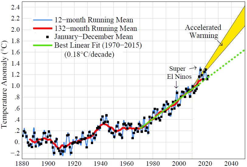
Fig. 19. Accelerated warming rate post-2010 (yellow area) if aerosol reductions approximately
double the net (GHG + aerosol) climate forcing. Upper and lower edges of the yellow area are
0.36 and 0.27°C per decade warming rates.
Aerosol climate forcing
Aerosol climate forcing is larger than the recent (AR6) IPCC estimate. Aerosols probably
provided a significant climate forcing prior to the industrial revolution. We know of no other
persuasive explanation for the absence of significant global warming during the past 6000 years
(Fig. 8), a period in which the GHG forcing increased 0.5 W/m 2 . Climate models that do not
incorporate a growing negative aerosol forcing yield significant warming in that period, 139 a
warming that, in fact, did not occur. Negative aerosol forcing, increasing as civilization
33
developed and population grew, should be expected. As humans burned fuels at a growing rate –
wood and other biomass for millennia and fossil fuels in the industrial era – aerosols as well as
GHGs were an abundant, growing, biproduct. The wood-burning aerosol source has continued in
modern times. 140 GHGs are long-lived and accumulate, so their forcing eventually dominates
unless aerosol emissions grow higher and higher – the Faustian bargain. 85
We conclude that peak aerosol climate forcing – in the first decade of this century – was of a
(negative) magnitude of at least 1.5-2 W/m 2 . We estimate that the GHG plus aerosol climate
forcing during the period 1970-2010 grew +0.3 W/m 2 per decade (+0.45 from GHG, – 0.15 from
aerosols), which produced observed warming of 0.18°C per decade. With current policies, we
expect climate forcing for a few decades post-2010 to increase 0.5-0.6 W/m 2 per decade and
produce global warming at a rate at least +0.27°C per decade. In that case, global warming
should reach 1.5°C by the end of the 2020s and 2°C by 2050 (Fig. 19).
Summary of present climate status
GHG climate forcing imagined by Charney, Tyndall and other greenhouse giants 1 is no longer
imaginary: the GHG climate forcing increase since 1750 (~4.1 W/m 2 ) is equivalent to 2×CO 2 .
GHG forcing is now growing by almost 0.5 W/m 2 per decade (Fig. 15) and it is no longer partly
offset by increasing aerosols. The situation that E.E. David warned about is now coming into
play. As David noted, a system with long delay and amplifying feedbacks can break down,
unless “anticipation is built into the loop.” Required anticipation was development of energies
that produce no GHGs. Instead, the fossil fuel industry, subsidized by the government, developed
fracking to enlarge the pool of available fossil fuels.
Climate’s delayed response allowed policy procrastination, as the impacts of climate change
were not glaringly apparent to the public. The designated scientific authority (IPCC), relying
primarily on climate models, continued for decades to report a broad range for estimated global
climate sensitivity: 1.5-4.5°C for 2×CO 2 , with non-negligible possibility that it was less than
1.5°C. Meanwhile, Earth’s paleoclimate history tells a clearer story: climate sensitivity is near
the high end of that long-time estimated range. Another excuse for inaction was hope that large
climate impacts will be delayed until humanity is wealthier and able to mitigate problems. Hope
of lethargic climate was based in part on the millennial time scale of large paleoclimate changes
(Fig. 2). However, the timescale of those paleoclimate changes results more from the timescale
of the forcings, rather than an inherent lethargy of the climate system. Our second perspective
article – Sea Level Rise in the Pipeline 93 – concludes, as outlined already, 15 that exponential
increase of sea level rise to at least several meters is likely if high fossil fuel emissions continue.
Specifically, it is concluded that the time scale for loss of the West Antarctic ice sheet and
multimeter sea level rise would be of the order of a century, not a millennium. Eventual impacts
would include loss of coastal cities and flooding of regions such as Bangladesh, the Netherlands,
a substantial portion of China, and the state of Florida in the United States. For practical
purposes, the losses would be permanent. Such outcome could be locked in soon, which creates
an urgency to understand the physical system better and to take major steps to reduce the human-
made drive of global warming.
34
Rapid human-made global warming that began in about 1970 (Fig. 12) has taken climate far out
of the Holocene range, the climate to which civilization is adapted, but ocean and ice sheet
inertia still allow reasoned policy response that may preserve a bright future for young people
and future generations. The basic requirement to preserve shorelines is return to a climate no
warmer than the mid-20 th century, possibly a bit cooler. This cooler climate will also address
other problems such as overheating of low latitudes and increasing regional climate extremes.
Policy implications
Climate science has exposed a crisis that the world is loath to fully appreciate. Delayed response
of the climate system has allowed huge global warming to build up in the pipeline. Humanity is
now entering the period of consequences. Scientists – as informed witnesses of ongoing efforts
of the world to deal with climate change via the Framework Convention and IPCC processes –
have the opportunity, indeed, the obligation, to assess the present course of those efforts.
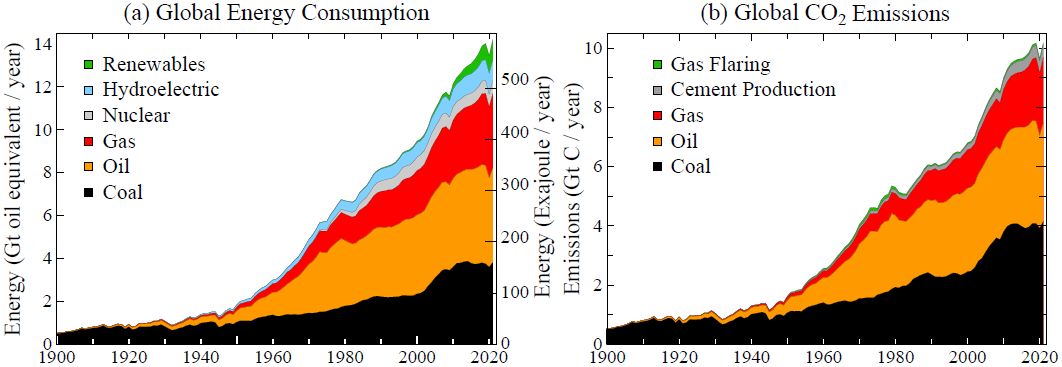
Fig. 20. Global energy consumption and CO 2 emissions (Hefner et al. 141 and BP 142 ; see text).
Fossil fuels powered the industrial revolution as the energy source that raised living standards in
much of the world. Fossil fuels continue to provide most of the world’s energy (Fig. 20a) and
produce most of the CO 2 emissions (Fig. 20b). Fossil fuel reserves and recoverable resources are
more than enough to provide most of the world’s energy for the rest of this century, 143 and
barring new effective policies they will continue to do so – and they will continue to drive global
warming at an unprecedented rate that we now understand is exceedingly dangerous.
Climate policy under the Framework Convention is demonstrably flawed. Empirical data (Fig.
20) confirm that as long as fossil fuel pollution can be dumped in the air free of charge,
agreements such as the 1997 Kyoto Protocol and 2015 Paris Agreement have little effect on
global emissions. 144 The reason is clear: much of the world is in early or middle stages of
economic development. Energy is required to raise living standards, and fossil fuels continue to
be the most convenient, affordable source for that energy. Thus growth of emissions is occurring
in the developing world (Fig. 21a), while the developed world is still the larger source of the
cumulative emissions (Fig. 21b) that drive climate change. 145,146 Thus, exhortations at annual
COP meetings, imploring each nation to set tighter emission targets, have little effect on global
35
emissions, as is blatantly apparent in the yawning gap between reality and the RCP2.6 scenario
(Fig. 15) designed to keep global warming below 2°C.
Moreover, a 2°C (or 1.5°C) target is more politically-based or practically-based than science-
based. The science-based target, we assert, should be return to Holocene climate, the climate in
which civilization developed and is adapted to. We must avoid passing points-of-no-return with
unacceptable consequences, such as loss of the West Antarctic ice sheet and thus loss of global
cities. That goal should also suffice for other unacceptable consequences, such as avoiding
unlivable conditions in the tropics and subtropics. A crucial issue that science must address is the
magnitude and duration of Holocene-overshoot that can occur without passing points-of-no-
return. We are already into overshoot territory and greater overshoot is in the offing.
Given the situation that we have allowed to develop, three actions now seem to be essential.
First, a rising global price on GHG emissions must underly energy and climate policies, with
enforcement by border duties on products from countries that do not have an internal carbon fee
or tax. Public buy-in and maximum effectiveness require the collected funds to be distributed to
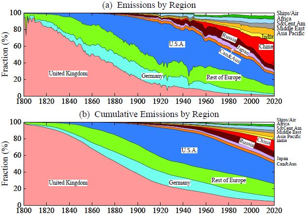
Fig. 21. Fossil fuel CO 2 emissions by nation or region as a fraction of global emissions. Data
sources: Heffner et al. 141 for 1751-2017 concatenated with BP 142 for 2018-2020.
the public, an approach that helps address global wealth disparities. Economists in the U.S.
overwhelming support such a carbon fee-and-dividend; 147 college and high school students, who
have much at stake, join in advocacy. 148 The science rationale for a rising carbon price with a
level playing field for energy efficiency, renewable energies, nuclear power, and all innovations
has long been understood, but not achieved. Instead, fossil fuels and renewable energy are
36
heavily subsidized, including use of “renewable portfolio standards” that allow utilities to pass
added costs to consumers. Nuclear energy has thus been relatively disadvantaged and excluded
as a “clean development mechanism” under the Kyoto Protocol, based in part on myths about
damage caused by nuclear energy that are not supported by scientific facts. 149 A rising carbon fee
is an underlying strategy to develop a mix of electricity sources needed to achieve rapid
decarbonization, low cost, and reliability of the energy system.
Second, human-made geoengineering of Earth’s climate must be rapidly phased out. The best
measure of geoengineering is Earth’s energy imbalance (EEI), which has reached a level of at
least 0.9 W/m 2 averaged over the solar cycle (equivalent to the energy of 600,000 Hiroshima
atomic bombs per day) with most of the excess energy heating the ocean and melting ice.
Realistic phasedown of emissions alone cannot remove this imbalance in less than several
decades (cf. Fig. 15 and discussion thereof), which may be too slow to avoid locking in loss of
the West Antarctic ice sheet and sea level rise of several meters. Removal of human-made GHGs
from the air will be spurred by a carbon price, but GHG removal sufficient to reduce EEI to zero
may require decades, if it is even feasible. Given that GHG forcing is still rising rapidly, highest
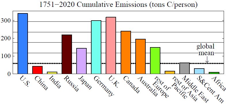
Fig. 22. Cumulative per capita national fossil fuel emissions. 150
priority must be given to phasing down emissions. However, given that GHG forcing is already 4
W/m 2 , it may be necessary to temporarily affect EEI via solar radiation management (SRM), if
the world is to avoid disastrous consequences, including large sea level rise. Risks of such
intervention must be defined, as well as risks of no intervention. Thus the U.S. National
Academy of Sciences recommends research on SRM. 151 An example of SRM is injection of
atmospheric aerosols at high southern latitudes, which global simulations suggest would cool the
Southern Ocean at depth and limit melting of Antarctic ice shelves. 15,152 The most innocuous
aerosols may be salt or fine salty droplets extracted from the ocean and sprayed into the air by
autonomous sailboats. 153 This approach has been discussed for potential use on a global scale, 154
but even use limited to high latitudes in the Southern Hemisphere will require extensive research
and forethought to avoid unintended adverse effects. 155 The present decade may be the last
opportunity to develop the knowledge, technical capability, and political will for the actions that
are needed to save global coastal regions from long-term inundation.
Third, effective global cooperation is needed to achieve the required reduction of GHG climate
forcing over the next several decades. Higher income countries – most of them in the West – are
responsible for most of the cumulative fossil fuel CO 2 emissions (Fig. 21b and Fig. 22), which
37
are the main drive for global warming, 145,146 even though the West constitutes a small fraction of
global population. De facto cooperation between the West and China drove down the price of
renewable energy, especially solar power, and further cooperation is needed to develop emission-
free technologies for the rest of the world that will be the source of most future GHG emissions
(Fig. 21a). Given China’s huge demand for carbon-free energy if its coal use is to be displaced,
China-U.S. cooperation in development of modern nuclear power was proposed, but then
stymied by U.S. prohibition of technology transfer. 156 Competition is normal, but if there is a
will it can be managed, reaping the benefits of cooperation over confrontation. 157 Of late, priority
seems to be given to economic and military hegemony, despite recognition of the long-term
existential threat posed by climate change. It is important to not foreclose the possibility of return
to a more ecumenical perspective of our shared future. In this situation, scientists can improve
global prospects by maintaining and expanding international cooperation. Public and political
awareness of the gathering climate storm will grow this decade as climate anomalies increase, so
it is important to improve scientific understanding and lay groundwork for effective actions.
38
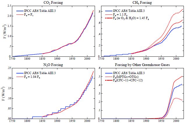
Fig. S1. GHG forcings. IPCC from AR6 Table AIII.3. Our forcings from Eq. (3) and Table 1.
SUPPORTING MATERIAL
1. GHG forcing formulae and comparison with IPCC forcings
Formulae (Table 1) for adjusted forcing, F a , were numerical fits 37 to 1-D calculations with the GISS GCM
radiation code using the correlated k-distribution method. 38 Gas absorption data were from high spectral
resolution laboratory data. 39 These F a were converted to F e via GCM calculations that include 3-D effects,
as summarized in Eq. (3), where the coefficients are from Table 1 of Efficacy. 31 The factor 1.45 for CH 4
includes the effect of CH 4 change on stratospheric H 2 O and tropospheric O 3 . We assume that CH 4 is
responsible for 45% of the O 3 change. 40 The remaining 55% of the O 3 forcing is obtained by multiplying
the IPCC AR6 O 3 forcing (0.47 W/m 2 in 2019) by 0.55 and by 0.82, where the latter factor is the efficacy
that converts F a to F e . The non-CH 4 portion of the O 3 forcing is thus 0.21 W/m 2 in 2019. The time-
dependence of this portion of the O 3 forcing is from Table AIII.3 in IPCC AR6. MPTGs and OTGs are
Montreal Protocol Trace Gases and Other Trace Gases. 41 An updated list of these gases and a table of
their annual forcings since 1992 are available as are earlier data. 42

39

Fig. S2. Test of accuracy of 2-term approximation for forcing by the three gases.
2. Approximation for N 2 O forcing
CO 2 and CH 4 are well-preserved in ice cores. However, the N 2 O record is corrupted in some time
intervals by chemical reactions with dust particles in the ice core. For such intervals we
approximate the N 2 O forcing by increasing the sum of CO 2 and CH 4 forcings by 12%, i.e., we
approximate the forcing for all three gases as 1.12×[F(CO 2 ) + F(CH 4 )]. The accuracy of this
approximation is checked in Fig. S2 via computations for the past 132 ky, when data are
available for all three gases from the multi-core composite of Schilt et al. 56

Fig. S3. Climate forcings provided in current IPCC report 13 for GHGs plus aerosols and for all
human-made forcings, i.e., excluding only volcano and solar forcings.
3. Comparison of GHG + Aerosol forcing with All Human-Made forcing
IPCC all human-made forcings include land-use effects and contrails, which have large relative
uncertainties. The forcings in Fig. S3 are those provided by IPCC (cf. Annex III of the current
IPCC physical sciences report). 13
40
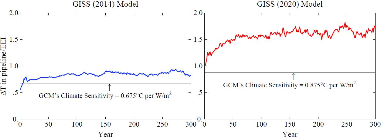
Fig. S4. Ratio of warming in the pipeline to EEI, (Teq – T)/EEI, for the first 300 years after
instant doubling of CO 2 for (a) GISS (2014) model and (b) GISS (2020) model.
4. Global warming in the pipeline: Green’s function calculations
Global warming in the pipeline (∆Tpl) after a CO 2 doubling is the portion of the equilibrium
response (Teq) that remains to occur at time t, i.e., ∆Tpl = Teq – T(t). If EEI were equivalent to a
climate forcing, warming in the pipeline would be the product of EEI and climate sensitivity (°C
per W/m 2 ), i.e., warming in the pipeline would be EEI ×ECS/4, where we have approximated the
2×CO 2 forcing as 4 W/m 2 .
Fig. S4 shows the 2×CO 2 results for the GISS (2014) and GISS (2020) GCMs. EEI is not a good
measure of the warming in the pipeline, especially for the newer GISS model. The warming in
the pipeline for the GISS (2014) model is typically ~30% larger than implied by EEI and ~90%
larger in the GISS (2020) model. If these results are realistic, they suggest that reduction of the
human-made climate forcing by an amount equal to EEI will leave a planet that is still pumping
heat into the ocean at a substantial rate.
Real-world climate forcing is added year-by-year with much of the GHG growth in recent years,
which Fig. 4 suggests will limit the discrepancy between actual warming in the pipeline and that
inferred from EEI. Thus, we also make Green’s function calculations of global temperature and
EEI for 1750-2019 for GHG plus IPCC aerosol forcings. Green’s function calculations are
useful, with a caveat noted below, for quantities for which the response is proportional to the
forcing. We calculate T G (t) using Eq. (4) and EEI G (t) using
EEI G (t) = ʃ [1 – R EEI (t)] × [dF(t)/dt] dt, (S1)
where R EEI (Fig. 5b) is the EEI response function (% of equilibrium response) and dF is forcing
change per unit time. Integrations begin in 1750, when we assume Earth was in energy balance.
The results (Fig. S5) show that the excess warming in the pipeline (excess over expectations
based on EEI) is reduced to 15-20% for the GISS (2014) model, but it is still 70-80% for the
GISS (2020) model. This topic thus seems to warrant further examination, but it is beyond the
scope of our present paper.
41

Fig. S5. Ratio of warming in the pipeline to EEI, (Teq – T G )/EEI G , in response to GHG and
IPCC aerosol forcing for the period 1750-2019 using the response functions for the GISS (2014)
model (left) and (b) GISS (2020) model (right).
The first matter to investigate is the cause of the ultrafast response of EEI (Fig. 5 of the main
paper), which could be done via the model diagnostics discussed in that section of our paper. If
the large difference between the EEI response functions of the two GISS models is related to
supercooled cloud water, Fig. 1 of the Kelley et al. paper 34 suggests that the real-world effect
may fall between that of the two models. If the higher climate sensitivity of the GISS (2020)
model is related to this cloud water phase problem, more realistic treatment of the latter may
yield a climate sensitivity between that of the 2014 and 2020 models.
If real world climate sensitivity for 2×CO 2 is near 4°C or higher, as we have concluded, the total
cloud feedback is likely to be even higher than that of the GISS (2020) model. We suggest that it
would be useful to calculate response functions for other models, especially models with high
climate sensitivity, to help analyze feedbacks and to allow inexpensive climate simulations for
arbitrary forcing scenarios. One major caveat: we have used a single response function calculated
for 2×CO 2 . Especially in view of cloud feedbacks, it seems likely that the response function for
aerosol forcing is different from that for CO 2 forcing, because most tropospheric aerosols exist
well below the clouds. Much might be learned from calculating response functions for GHGs,
tropospheric aerosols, stratospheric aerosols, and solar irradiance, for example.
The response functions for global temperature and EEI, for both the 2014 and 2020 models,
smoothed and unsmoothed, are available at
http://www.columbia.edu/~mhs119/ResponseFunctionTables/
DATA AVAILABILITY
"The data used to create the figures in this paper are available in the Zenodo repository,
at https://dx.doi.org/[doi]."
ACKNOWLEDGMENTS
We thank Eelco Rohling for inviting JEH to describe our perspective on global climate response
to human-made forcing. JEH began to write a review of past work, but a paper on the LGM by
42
Jessica Tierney et al. 23 and data on changing ship emissions provided by Leon Simons led to the
need for new analyses and division of the paper into two parts. We thank Jessica also for
pointing out the paper by Zhu et al. 83 , which independently identifies cloud drop microphysics at
cloud tops as key physics affecting climate sensitivity that can be constrained by paleoclimate
data. JEH designed the study and carried out the research with help of Makiko Sato; Larissa
Nazarenko provided data from GISS models and helped with analysis; Leon Simons provided
ship emission information and aided interpretations; Norman Loeb and Karina von Schuckmann
provided EEI data and insight about implications; Matthew Osman provided paleoclimate data
and an insightful review of the entire paper; Qinjian Jin provided simulations of atmospheric
sulfate and interpretations; all authors contributed to our prior research incorporated in the paper
and reviewed and commented on the manuscript.
All authors declare that they have no conflicts of interest. Climate Science, Awareness and
Solutions, which is directed by JEH and supports MS and PK is a 501(C3) non-profit supported
100% by public donations. Principal supporters in the past few years have been the Grantham
Foundation, Carl Page, Frank Batten, James and Krisann Miller, Peter Joseph, Ian Cumming,
Eric Lemelson, Gary and Claire Russell, Donald and Jeanne Keith Ferris, Aleksandar Totic,
Chris Arndt, Jeffrey Miller, Morris Bradley and about 150 more contributors to annual appeals.
1 Tyndall, J., On the absorption and radiation of heat by gases and vapours, Phil. Mag. 22, 169-194, 273-285, 1861.
2 Hansen, J.: draft Chapter 15 (Greenhouse Giants) of Sophie’s Planet, a book in preparation. Tyndall made the
greatest early contributions to understanding of “greenhouse” science, but Eunice Foote earlier investigated the role
of individual gases in affecting Earth’s temperature and speculated on the role of CO 2 in altering Earth’s
temperature. Draft Chapters 15, 16 (Farmers’ Forecast vs End-of-Century) and 17 (Charney’s Puzzle: How Sensitive
is Earth?) are permanently available here; criticisms are welcome.
3 Revelle, R., W. Broecker, H. Craig, C.D. Keeling, and J. Smagorinsky, President’s Science Advisory Committee,
Restoring the Quality of Our Environment, Appendix Y4 Atmospheric Carbon Dioxide, The White House,
November, 1965.
4 Charney, J., Arakawa, A., Baker, D., Bolin, B., Dickinson, R., Goody, R., Leith, C., Stommel, H. and Wunsch, C.:
Carbon Dioxide and Climate: A Scientific Assessment, Natl. Acad. Sci. Press, Washington, DC, 33p, 1979.
5 Nierenberg, W.A. (Chairman), Changing Climate: Report of the Carbon Dioxide Assessment Committee,
Washington, DC, National Academies Press, 519 pages, https://doi.org/10.17226/18714, 1983.
6 Hansen, J.E., and T. Takahashi (Eds.): Climate Processes and Climate Sensitivity. AGU Geophysical Monograph
29, Maurice Ewing Vol. 5. American Geophysical Union, 368 pp., 1984.
7 Hansen, J., A. Lacis, D. Rind, G. Russell, P. Stone, I. Fung, R. Ruedy and J. Lerner, Climate sensitivity: analysis of
feedback mechanisms, 130-163, in reference 6 (American Geographical Union Monograph 29).
8 David, E.E., Jr.: Inventing the Future: Energy and the CO 2 “Greenhouse “ Effect, in reference 6 (American
Geographical Union Monograph 29).
9 E.E. David, Jr. later became a global warming denier
10 Oreskes N, Conway E.: Merchants of Doubt: How a Handful of Scientists Obscured the Truth on Issues from
Tobacco Smoke to Global Warming. London: Bloomsbury, 2010.
11 History of the IPCC, accessed 15 June 2022.
12 United Nations: Framework Convention on Climate Change (UNFCCC), United Nations, New York, NY
(accessed at https://unfccc.int/process-and-meetings/what-is-the-united-nations-framework-convention-on-climate-
change), 1992.
13 IPCC, 2021: Climate Change 2021: The Physical Science Basis. Contribution of Working Group I to the Sixth
Assessment Report of the Intergovernmental Panel on Climate Change [Masson-Delmotte, V., P. Zhai, A. Pirani,
S.L. Connors, C. Péan, et al. (eds.)]. Cambridge University Press. In Press.
14 Hansen, J., M. Sato, P. Hearty, R. Ruedy, M. Kelley, V. Masson-Delmotte, G. Russell, G. Tselioudis, J. Cao, E.
Rignot, I. Velicogna, B. Tormey, B. Donovan, E. Kandiano, K. von Schuckmann, P. Kharecha, A.N. Legrande, M.
43
Bauer, and K.-W. Lo: Ice melt, sea level rise and superstorms: evidence from paleoclimate data, climate modeling,
and modern observations that 2 C global warming could be dangerous Atmos. Chem. Phys., 16, 3761-3812, 2016.
15 Hansen, J.: Foreword: uncensored science is crucial for global conservation, in DellaSala, D.A. (Ed.)
Conservation Science and Advocacy for a Planet in Peril, 451 pp., Elsevier, Amsterdam, Netherlands.
16 Lunt, D. J., Haywood, A. M., Schmidt, G. A., Salzmann, U., Valdes, P. J., and Dowsett, H. J.: Earth system
sensitivity inferred from Pliocene modelling and data, Nat. Geosci. 3, 60–64, 2010.
17 Rohling, E.J., et al. (PALAEOSENS Project Members): Making sense of palaeoclimate sensitivity, Nature
491(7426), 683–691, 2012.
18 Caballero, R., M. Huber, State-dependent climate sensitivity in past warm climates and its implications for future
climate projections: Proc. Natl. Acad. Sci. U.S.A. 110, 14162–14167, 2013.
19 Inglis, G.N. et al.: Global mean surface temperature and climate sensitivity of the early Eocene Climatic Optimum
(EECO), Paleocene–Eocene Thermal Maximum (PETM), and latest Paleocene, Clim. Past 16, 1953–1968, 2020.
20 Turner, S.K.: Constraints on the onset duration of the Paleocene–Eocene Thermal Maximum, Phil. Trans. Roy.
Soc. A 376, 20170082, 2018.
21 CLIMAP project members: Seasonal reconstruction of the Earth’s surface at the last glacial maximum, Geol. Soc.
Amer., Map and Chart Series, No. 36, 1981.
22 Rind, D. and D. Peteet: Terrestrial conditions at the last glacial maximum and CLIMAP sea-surface temperature
estimates: Are they consistent? Quat. Res., 24, 1-22, 1985, doi:10.1016/0033-5894(85)90080-8.
23 Tierney, J.E., J. Zhu, J. King, S.B. Malevich, G.J. Hakim and C.J. Poulson: Glacial cooling and climate sensitivity
revisited, Nature 584, 569-573, 2020.
24 Osman, M.B., J.E. Tierney, J. Zhu, R. Tardif, G.J. Hakim, J. King and C.J. Poulson: Globally resolved surface
temperatures since the Last Glacial Maximum, Nature 599, 239-244, 2021.
25 At maximum LGM cooling, i.e., at 18 ky BP, the cooling is ~7°C (Osman et al. , 2021; Tierney, priv. comm.).
26 Seltzer, A.M., J. Ng, W. Aeschbach, R. Kipfer, J.T. Kulongoski, J.P. Severinghaus and M. Stute, Widespread six
degrees Celsius cooling on land during the Last Glacial Maximum, Nature 593, 228-232, 2021.
27 IPCC, 2014: Climate Change 2014: Synthesis Report. Contribution of Working Groups I, II and III to the Fifth
Assessment Report of the Intergovernmental Panel on Climate Change [Core Writing Team, R.K. Pachauri and L.A.
Meyer (eds.)]. IPCC, Geneva, Switzerland, 151 pp.
28 Sherwood, S.C., M.J. Webb, J.D. Annan, K.C. Armour, P.M. Forster, J.C. Hargreaves, et al.: An assessment of
Earth’s climate sensitivity using multiple lines of evidence, Rev. Geophys. 58, e2019RG000678, 2020.
29 Baggenstos, D., Häberli, M., Schmitt, J., Shackleton, S. A., Birner, B., Severinghaus, J. P., Kellerhals, T., and
Fischer, H.: Earth's radiative imbalance from the Last Glacial Maximum to the present, Proc. Natl. Acad. Sci. USA,
116, 14881, 2019.
30 Myhre, G., D. Shindell, F.-M. Bréon, W. Collins, J. Fuglestvedt, J. Huang, D. Koch, J.-F. Lamarque, D. Lee, B.
Mendoza, T. Nakajima, A. Robock, G. Stephens, T. Takemura and H. Zhang, 2013: Anthropogenic and Natural
Radiative Forcing. In: Climate Change 2013: The Physical Science Basis. Contribution of Working Group I to the
Fifth Assessment Report of the Intergovernmental Panel on Climate Change [Stocker, T.F., D. Qin, G.-K. Plattner,
M. Tignor, S.K. Allen, J. Boschung, A. Nauels, Y. Xia, V. Bex and P.M. Midgley (eds.)]. Cambridge University
Press, Cambridge, United Kingdom and New York, NY, USA.
31 Hansen, J., M. Sato, R. Ruedy, L. Nazarenko, A. Lacis, G.A. Schmidt, G. Russell, et al., Efficacy of climate
forcings. J. Geophys. Res. 110, D18104, 2005.
32 Lohmann, U., L. Rotstayn, T. Storelvino, A. Jones, S. Menon, J. Quass, A.M.L. Ekman, D. Koch and R. Ruedy:
Total aerosol effect: radiative forcing or radiative flux perturbation? Atmos. Chem. Phys. 10, 3235-3246, 2010.
33 Eyring, V., Bony, S., Meehl, G. A., Senior, C. A., Stevens, B., Stouffer, R. J., & Taylor, K. E. (2016). Overview
of the Coupled Model Intercomparison Project Phase 6 (CMIP6) experimental design and organization.
Geoscientific Model Devel. 9(5), 1937–1958, https://doi.org/10.5194/gmd-9-1937-2016.
34 Kelley, M., G.A. Schmidt, L. Nazarenko, S.E. Bauer, R. Ruedy, G.L. Russell, et al., GISS-E2.1: Configurations
and climatology. J. Adv. Model. Earth Syst., 12, no. 8, e2019MS002025, 2020.
35 Miller, R.L., G.A. Schmidt, L. Nazarenko, S.E. Bauer, M. Kelley, R. Ruedy, G.L. Russell, et al.: CMIP6 historical
simulations (1850-2014) with GISS-E2.1. J. Adv. Model. Earth Syst., 13, no. 1, e2019MS002034, 2021.
36 The specific GISS (2020) model is described as GISS-E2.1-G-NINT in published papers; NINT (noninteractive)
signifies that the models use specified GHG and aerosol amounts.
37 Hansen, J., M. Sato, R. Ruedy, A. Lacis, and V. Oinas: Global warming in the twenty-first century: An alternative
scenario. Proc. Natl. Acad. Sci., 97, 9875-9880, 2000.
38 Lacis, A.A., and V. Oinas, 1991: A description of the correlated k distributed method for modeling nongray
gaseous absorption, thermal emission, and multiple scattering in vertically inhomogeneous atmospheres. J. Geophys.
Res., 96, 9027-9063, doi:10.1029/90JD01945.
44
39 Rothman, L., Rinsland, C., Goldman, A., Massie, S., Edwards, D., Flaud, J., Perrin, A., Camy-Peyret, C., Dana,
V., Mandin, J., et al.: The HITRAN molecular spectroscopic database and HAWKS (HITRAN Atmospheric
Workshation) 1996 edition, J. Quan. Spec. Rad. Trans. 60, 665–710, 1998.
40 Prather, M., and D. Ehhalt: Atmospheric chemistry and greenhouse gases, Chap. 4, pp. 239– 287, in Climate
Change 2001: The Scientific Basis, edited by J. T. Houghton et al., Cambridge Univ. Press, New York, 2001.
41 Hansen, J. and M. Sato. Greenhouse gas growth rates. Proc. Natl. Acad. Sci. 101, 16109-16114, 2004.
42 Links to MPTG and OTG data: www.columbia.edu/~mhs119/GHGs/TG_F.1900-1990.txt and
www.columbia.edu/~mhs119/GHGs/TG_F.1992-2020.txt
43 Jouzel, J., Masson-Delmotte, V., Cattani, O., Dreyfus, G., Falourd, S., Hoffmann, G., Minster, B., Nouet, J.,
Barnola, J.M., Chappellaz, et al.: Orbital and millennial Antarctic climate variability over the past 800,000 years,
Science, 317, 793-796, 2007.
44 Luthi, D., Le Floch, M., Bereiter, B., Blunier, T., Barnola, J.M., Siegenthaler, U., Raynaud, D., Jouzel, J., Fischer,
H., Kawamura, K., and Stocker, T.F.: High-resolution carbon dioxide concentration record 650,000-800,000 years
before present, Nature, 453, 379-382, 2008.
45 Hays, J.D., J. Imbrie and N.J. Shackleton: Variation in the Earth’s orbit: pacemaker of the ice ages, Science, 194,
1121-1132, 1976.
46 Lorius, C., J. Jouzel, D. Raynaud, J. Hansen, and H. Le Treut: The ice-core record: Climate sensitivity and future
greenhouse warming. Nature, 347, 139-145, 1990.
47 Zachos, J., Pagani, M., Sloan, L., Thomas, E., and Billups, K.: Trends, rhythms, and aberrations in global climate
65 Ma to present. Science, 292, 686-693, 2001.
48 Hansen, J., M. Sato, P. Kharecha, G. Russell, D.W. Lea, and M. Siddall: Climate change and trace gases. Phil.
Trans. Royal. Soc. A, 365, 1925-1954, 2007.
49 MARGO Project Members. Constraints on the magnitude and patterns of ocean cooling at the Last Glacial
Maximum. Nat. Geosci. 2, 127–132, 2009.
50 Hansen, J., L. Nazarenko, R. Ruedy, M. Sato, J. Willis, A. Del Genio, D. Koch, A. Lacis, K. Lo, S. Menon, T.
Tovakov, Ju. Perlwitz, G. Russell, G.A. Schmidt, and N. Tausnev: Earth's energy imbalance: Confirmation and
implications. Science 308, 1431-1435, 2005.
51 It is often said that glacial terminations (at intervals ~100,000 years in Fig. 2) occur when Earth orbital parameters
produce maximum summer insolation at the latitudes of Northern Hemisphere ice sheets (e.g., Cheng, H., Edwards,
R.L., Broecker, W.S., Denton, G.H., Kong, X., Wang, Y., Zhang R. and Wang, X., Ice age terminations, Science
326, 248-252, 2009). However, close examination of termination dates shows that they occur at times of late Spring
(mid-May) maximum radiation anomalies (Reference 48). Maximum insolation anomaly in late Spring causes
meltwater induced darkening of the ice to occur as early in the year as possible, thus lengthening the melt season.
52 Ruddiman, W.F.: The anthropogenic greenhouse era began thousands of years ago, Clim. Change 61, 261-293,
2003.
53 Rohling, E.J., F.D. Hibbert, F.H. Williams, K.M. Grant, G. Marino, G.L. Foster, R. Hennekam, G.J. de Lange,
A.P. Roberts, J. Yu., J. M. Webster and Y. Yokoyama, Differences between the last two glacial maxima and
implications for ice-sheet, ō18O, and sea-level reconstructions, Quaternary Sci. Rev. 176, 1-28, 2017.
54 Hansen, J., M. Sato, P. Kharecha, K. von Schuckmann, D.J. Beerling, J. Cao, S. Marcott, V. Masson-Delmotte,
M.J. Prather, E.J. Rohling, J. Shakun, P. Smith, A. Lacis, G. Russell, and R. Ruedy: Young people's burden:
requirement of negative CO2 emissions. Earth Syst. Dynam., 8, 577-616, 2017.
55 Hoffman, J.S., Clark, P.U., Parnell, A.C., and He, F.: Regional and global sea-surface temperatures during the last
interglaciation, Science, 355(6322), 276-279, 2017.
56 Schilt, A., Baumgartner, M., Schwander, J., Buiron, D., Capron, E., Chappellaz, J., Loulergue, L., Schupach, S.,
Spahni, R., Fischer, H., and Stocker, T.F.: Atmospheric nitrous oxide during the last 140,000 years, Earth Planet.
Sci. Lett., 300, 33-43, 2010.
57 PGM → Eemian: CO 2 196 → to 272 ppm yields 1.82 W/m 2 ; CH 4 388 → 615 ppb yields 0.27 W/m 2 ; N 2 O 215 →
265 ppb yields 0.21 W/m 2 for total 2.30 W/m 2 . LGM → early Holocene: CO 2 191 → 261 ppm yields 1.72 W/m 2 ;
CH 4 374 → 527 ppb yields 0.19 W/m 2 ; N 2 O 204 → 259 ppb yields 0.24 W/m 2 for total 2.15 W/m 2 . LGM → late
Holocene: CO 2 191 → 275 ppm yields 2.00 W/m 2 ; CH 4 374 → 591 ppb yields 0.26 W/m 2 ; N 2 O 204 → 265 ppb
yields 0.26 W/m 2 for total 2.52 W/m 2 .
58 Schneider, T., J. Teixeira, C.S. Bretherton, F. Brient, K.G. Pressel, C. Achar and A.P. Siebesma: Climate goals
and computing the future of clouds, Nature Clim. Chan. 7, 3-5, 2017.
59 Kagiyama, M., P. Braconnot, S.P. Harrison, A.M. Haywood, J.H. Jungclaus, B.L. Otto-Bliesneret al.: The PMIP4
contribution to CMIP6 – Part 1: overview and over-arching analysis plan, Geosci. Model Dev. 11, 1033-1057, 2018.
60 Pincus, R., P.M. Forster and B. Stevens: The radiative forcing model intercomparison project (RFMIP):
experimental protocol for CMIP6, Geoscientific Model Devel. 9, 3447-3460, 2016.
45
61 Hegerl, G. C., Zwiers, F. W., Braconnot, P., Gillett, N. P., Luo, Y., Marengo Orsini, J. A., et al. (2007). Chapter 9:
Understanding and attributing climate change. In S. D. Solomon, et al. (Eds.), Climate change 2007: The physical
science basis. Contribution of Working Group I to the Fourth Assessment Report of the Intergovernmental Panel on
Climate Change. Cambridge, UK and New York, USA: Cambridge University Press.
62 Yoshimori, M., T. Yokohata and A. Abe-Ouchi: A comparison of climate feedback strength between CO 2
doubling and LGM experiments, J. Clim. 22, 3374-3395, 2009.
63 Stap, L.B., P. Kohler and G. Lohmann: Including the efficacy of land ice changes in deriving climate sensitivity
from paleodata, Earth Syst. Dynam. 10, 333-345, 2019.
64 Koppen, W.: Das geographische system der climate, in Handbuch der Klimatologie 1, part C, eds. W. Koppen and
G. Geiger, Boentraeger, Berlin, 1936.
65 Kohler, P., R. Bintanja, H. Fischer,F. Joos, R. Knutti, G. Lohmann and V. Masson-Delmotte: What caused Earth’s
temperature variations during the last 800,000 years? Data-based evidence on radiative forcing and constraints on
climate sensitivity, Quatern. Sci. Rev. 29, 129-145, 2010.
66 Rabineau, M., S. Berne, J.L. Oliver, D. Aslanian, F. Guillocheau, and P. Joseph: Paleo sea levels reconsidered
from direct observation of paleoshoreline position during Glacial Maxima (for the last 500,000 yr). Earth Planet.
Sci. Lett. 252, 119-137, 2006.
67 Hansen, J., M. Sato, P. Kharecha, D. Beerling, R. Berner, V. Masson-Delmotte, M. Pagani, M. Raymo, D. Royer,
and J.C. Zachos: Target atmospheric CO 2 : Where should humanity aim? Open Atmos. Sci. J. 2, 217-231, 2008.
68 Ruth, U., Barnola, J.M., Beer, J., Bigler, M., Blunier, T. Castellano, E., Fischer, H., Fundel, F., Huybrechts, P.,
Kaufmann, P., Kipfstuhl, S., Lambrecht, A., Morganti, A., Oerter, H., Parrenin, F., Rybak, O., Severi, M., Udisti, R.,
Wilhelms, F., and Wolff, E.: EDML1: a chronology for the EPICA deep ice core from Dronning Maud Land,
Antarctica, over the last 150 000 years, Clim. Past, 3, 549-574, 2007.
69 Bryan, K., F.G. Komro, S. Manabe and M.J. Spelinan, Transient climate response to increasing atmospheric
carbon dioxide, Science, 215, 56-58, 1982.
70 Hansen, J., G. Russell, A. Lacis, I. Fung, D. Rind, and P. Stone: Climate response times: dependence on climate
sensitivity and ocean mixing. Science, 229, 857-859, 1985.
71 Hansen J Climate Threat to the Planet, American Geophysical Union, San Francisco, California, 17 December
2008, http://www.columbia.edu/~jeh1/2008/AGUBjerknes20081217.pdf. (3 December 2022, date last accessed).
72 Tom Delworth (NOAA Geophysical Fluid Dynamics Laboratory), Gokhan Danabasoglu (National Center for
Atmospheric Research), and Jonathan Gregory (UK Hadley Centre) provided long 2×CO 2 runs of GCMs of these
leading modeling groups. All three models had response times as slow or slower than the GISS GCM.
73 Yr 1 (no smoothing), yr 2 (3-yr mean), yr 3-12 (5-yr mean), yr 13-300 (25-yr mean), yr 301-5000 (101-yr mean).
74 Schmidt, G.A., M. Kelley, L. Nazarenko, R. Ruedy, G.L. Russell, et al., Configuration and assessment of the
GISS ModelE2 contributions to the CMIP5 archive. J. Adv. Model. Earth Syst., 6, 141-184, 2014.
75 The GISS (2014) model is labeled as GISS-E2-R-NINT and GISS (2020) as GISS-E2.1-G-NINT in published
papers, where NINT (noninteractive) signifies that the models use specified GHG and aerosol amounts.
76 Prather, M. J.: Numerical advection by conservation of second order moments. J. Geophys, Res. 91, 6671–6680,
1986.
77 Romanou, A., Marshall, J., Kelley, M., & Scott, J., Role of the ocean's AMOC in setting the uptake efficiency of
transient tracers. Geophysical Research Letters, 44, 5590–5598, 2017.
78 von Schuckmann, K., L. Cheng, M.D. Palmer, J. Hansen et al.: Heat stored in the Earth system: where does the
energy go?, Earth System Science Data 12, 2013-2041, doi:10.5195/essd-12-2013-2020, 2020.
79 Loeb, N. G., Johnson, G. C., Thorsen, T. J., Lyman, J. M., Rose, F. G., & Kato, S., Satellite and ocean data reveal
marked increase in Earth’s heating rate, Geophys. Res. Lett. 48, e2021GL093047, 2021.
80 See diagram (Fig. 4) of Hansen, J., D. Johnson, A. Lacis, S. Lebedeff, P. Lee, D. Rind, and G. Russell: Climate
impact of increasing atmospheric carbon dioxide. Science, 213, 957-966, 1981 for illustration of how solar, thermal
and dynamical fluxes adjust to instantaneous doubling of atmospheric CO 2 .
81 Kamae, Y., M. Watanabe, T. Ogura, M. Yoshimori and H. Shiogama: Rapid adjustments of cloud and
hydrological cycle to increasing CO 2 : a review, Curr. Clim. Chan. Rep 1, 103-113, 2015.
82 Zelinka, M.D., T.A. Myers, D.T. McCoy, S.Po-Chedley, P.M. Caldwell, P. Ceppi, S.A. Klein and K.E. Taylor,
Causes of higher climate sensitivity in CMIP6 models, Geophys. Res. Lett. 47, e2019GL085782, 2020.
83 Zhu, J., Otto-Bliesner, B. L., Brady, E. C., Gettelman, A., Bacmeister, J. T., Neale, R. B., et al:. LGM
paleoclimate constraints inform cloud parameterizations and equilibrium climate sensitivity in CESM2. J. Adv. Mod.
Earth Sys., 14, e2021MS002776, 2022.
84 See Supporting Material for links to GHG and response function data.
85 Hansen, J., 2009: Storms of My Grandchildren, Bloomsbury, New York, 320 pages.
86 World Health Organization, Ambient (outdoor) air pollution, Fact Sheet, 22 September 2021.accesed 2022.06.23.
46
87 Vimeux F, K.M. Cuffey and J. Jouzel, New insights into Southern Hemisphere temperature changes from Vostok
ice cores using deuterium excess correction, Earth Planet Sci. Lett. 203, 829-43, 2002.
88 Petit, J.R., J. Jouzel, D. Raynaud, et al. Climate and atmospheric history of the past 420,000 years from the
Vostok ice core, Antarctica, Nature 399, 429-36, 1999.
89 Hansen, J., R. Ruedy, M. Sato, and K. Lo: Global surface temperature change. Rev. Geophys., 48, RG4004, 2010.
90 Lenssen, N.J.L., G.A. Schmidt, J.E. Hansen, M.J. Menne, A. Persin, R. Ruedy, and D. Zyss, 2019: Improvements
in the GISTEMP uncertainty model, J. Geophys. Res. Atmos., 124(12), 6307-6326, 2019.
91 Tardiff, R., G.J. Hakim, W.A. Perkins, K.A. Horlick, M.F. Erb, J. Emile-Geay, D.M. Anderson, E.J. Steig and D.
Noone, Last Millenium Reanalysis with an expanded proxy database and seasonal proxy modeling, Clim. Past 15,
1251-1273, 2019.
92 Buizert, C. T. J. Fudge, W. H. G. Roberts, E. J. Steig, S. Sherriff-Tadano, C. Ritz, E. Lefebvre, et al.: Antarctic
surface temperature and elevation during the Last Glacial Maximum, Science 372 (6546), 1097-1101, 2021.
93 Hansen, J. et al.: Sea level rise in the pipeline, in preparation for submission to Oxford Open Climate Change.
94 Shakun, J.D., P.U.Clark, F. He, S.A. Marcott, A.C. Mix, Z. Liu, B. Otto-Bliesner, A. Schmittner and E. Bard:
Global warming preceded by increasing carbon dioxide concentrations during the last deglaciation, Nature 484, 49-
54, 2012.
95 Marcott, S. A., Shakun, J. D., Clark, P. U., and Mix, A. C.: A reconstruction of regional and global temperature
for the last 11,300, Science 339, 1198-1201, 2013.
96 Ruddiman, W.F., D.Q. Fuller, J.E. Kutzbach, P.C. Tzedakis, J.O. Kaplan, E.C. Ellis, S.J. Vavrus, C.N. Roberts, R.
Fyfe, F. He, C. Lemmon and J. Woodbridge: Late Holocene climate: natural or anthropogenic? Rev. Geophys. 54,
93-118, 2016.
97 https://commons.wikimedia.org/wiki/File:Post-Glacial_Sea_Level.png
98 Barber, B. Resistance by scientists to scientific discovery, Science 134, 596-602, 1961.
99 Hoffman, P.F., A.J. Kaufman, G.P. Halverson and D.P. Schrag: A Neoproterozoic Snowball Earth, Science 281,
1342-1346, 1998.
100 Alvarez, L.,W. Alvarez, F. Asaro and H. Michel: Extraterrestrial Cause for the Cretaceous-Tertiary
Extinction, Science 208, 1095–1108, 1980.
101 Mishchenko, M.I., B. Cairns, G. Kopp, C.F. Schueler, B.A. Fafaul, J.E. Hansen, R.J. Hooker, T. Itchkawich, H.B.
Maring, and L.D. Travis, 2007: Accurate monitoring of terrestrial aerosols and total solar irradiance: Introducing the
Glory mission. Bull. Amer. Meteorol. Soc., 88, 677-691, 2007.
102 Monthly updates of global temperature and related data at http://www.columbia.edu/~mhs119/Temperature/
103 Day, J.W., J.D. Gunn, W.J. Folan, A. Yaniz-Arancibia and B.P Horton: Emergence of complex societies after sea
level stabilized, EOS, Trans. Amer. Geophys. Union 88(15), 169-170, 2007.
104 Riser, S. C., Freeland, H. J., Roemmich, D., Wijffels, S., Troisi, A., Belbéoch, M., Gilbert, D., Xu, J., Pouliquen,
S., Thresher, A., Le Traon, P.-Y., Maze, G., Klein, B., Ravichandran, M., Grant, F., Poulain, P.-M., Suga, T., Lim,
B., Sterl, A., and Jayne, S. R.: Fifteen years of ocean observations with the global Argo array, Nat. Clim. Change 6,
145–153, 2016. Argo web page (http://www.argo.ucsd.edu/).
105 Hansen, J., M. Sato, P. Kharecha, and K. von Schuckmann: Earth's energy imbalance and implications. Atmos.
Chem. Phys. 11, 13421-13449, 2011.
106 Koch, D., S.E. Bauer, A. Del Genio, G. Faluvegi, J.R. McConnell, S. Menon, R.L. Miller, D. Rind, R. Ruedy,
G.A. Schmidt and D. Shindell: Coupled aerosol-chemistry-climate twentieth-century model investigation: trends in
short-lived species and climate responses, J. Clim. 24, 2693-2714, 2011.
107 Novakov, T., Ramanathan, V., Hansen, J. E., Kirschstetter, T. W., Sato, M., Sinton, J. E., and Sathaye, J. A.:
Large historical changes of fossil-fuel black carbon aerosols, Geophys. Res. Lett., 30, 1324, 2003.
108 Knutti, R., Why are climate models reproducing the observed global surface warming so well? Geophys. Res.
Lett., 35, L18704, 2008.
109 In the absence of a response function from a GCM with ECS = 4°C, we use the normalized response function of
the GISS (2020) model and put λ = 1°C per W/m 2 in equation (4).
110 Forster, P., T. Storelvmo, K. Armour, W. Collins, J.-L. Dufresne, D. Frame, D.J. Lunt, T. Mauritsen, M.D.
Palmer, M. Watanabe, M. Wild, and H. Zhang: The Earth’s Energy Budget, Climate Feedbacks, and Climate
Sensitivity. In Climate Change 2021: The Physical Science Basis. Contribution of Working Group I to the Sixth
Assessment Report of the Intergovernmental Panel on Climate Change [Masson-Delmotte, V., P. Zhai, A. Pirani,
S.L. Connors, C. Péan, S. Berger, N. Caud, Y. Chen, L. Goldfarb, M.I. Gomis, M. Huang, K. Leitzell, E. Lonnoy,
J.B.R. Matthews, T.K. Maycock, T. Waterfield, O. Yelekçi, R. Yu, and B. Zhou (eds.)]. Cambridge University
Press, Cambridge, United Kingdom and New York, NY, USA, pp. 923–1054, 2021.
47
111 Bauer, S.E., K. Tsigaridis, G. Faluvegi, M. Kelley, K.K. Lo, R.L. Miller, L. Nazarenko, G.A. Schmidt and J.
Wu: Historical (1850-2014) aerosol evolution and role on climate forcing using the GISS ModelE2.1 contribution to
CMIP6. J. Adv. Model. Earth Syst., 12(8), e2019MS001978, 2020.
112 The forcing in the “inferred aerosols” in Fig. 14 used for calculations in Fig. 13 is –1.8 W/m 2 in 2010, with a
change of – 0.2 W/m 2 in the period 1850-1880.
113 Wang, Z., Lin, L., Xu, Y., Che, H., Zhang, X., Zhang, H., Dong, W., Wang, C., Gui, K., and Xie, B.: Incorrect
Asian aerosols affecting the attribution and projection of regional climate change in CMIP6 models, Clim. Atmos.
Sci., 4, 2, https://doi.org/10.1038/s41612-020-00159-2, 2021.
114 Zheng, Y., Q. Zhang, D. Tong, S.J. Davis and K. Caldeira: Climate effects of China’s efforts to improve its air
quality, Environ. Res. Lett. 15, 104052, 2020.
115 International Maritime Organization (IMO), MEPC.176(58), Amendments to the annex of the protocol of 1997 to
amend the international convention for the prevention of pollution from ships, 1973, as modified by the protocol of
1978 relating thereto (Revised MARPOL, Annex VI), 2008.
116 Quaas, J., H. Jia, C. Smith, A.L. Albright, W. Aas, N. Bellouin, O. Boucher, M.Doutriaux-Boucher, P.M. Forster,
D. Grosvenor, S. Jenkins, Z. Klimont, N.G. Loeb, X. Ma, V. Naik, F. Paulot, P. Steir, M. Wild, G. Myhre and M.
Schulz: Robust evidence for reversal of the trend in aerosol effective climate forcing, Atmos. Chem. Phys. 22,
12,221-12,239, 2022.
117 Hansen, J., W. Rossow, B. Carlson, A. Lacis, L. Travis, A. Del Genio, I. Fung, B. Cairns, M. Mishchenko and M.
Sato: Low-cost long-term monitoring of global climate forcings and feedbacks, Clim. Change 31, 247-271, 1995.
118 Hansen, J., W. Rossow and I. Fung (eds.): Long-term monitoring of global climate forcings and feedbacks,
NASA Conference Publication 3234, 90 pages, 1993.
119 Bellouin, N., Quaas, J., Gryspeerdt, E., Kinne, S., Stier, P., Watson-Parris, D., et al.: Bounding global aerosol
radiative forcing of climate change, Rev. Geophys. 58, e2019RG000660, 2020.
120 Glassmeier, F., F. Hoffmann, J.S. Johnson, T. Yamaguchi, K.S. Carslaw and G. Feingold: Aerosol-cloud-climate
cooling overestimated by ship-track data, Science 371, 485-489, 2021.
121 Manshausen, P., D. Watson-Parris, M.W. Christensen, J.P. Jalkanen and P. Stier: Invisible ship tracks show large
cloud sensitivity to aerosol, Nature 610, 101-106, 2022.
122 Wall, C.J., J.R. Norris, A. Possner, D.T. McCoy, I.L. McCoy and N.J. Lutsko: Assessing effective radiative
forcing from aerosol-cloud interactions over the global ocean, Proc. Natl. Acad. Sci. USA 119, e2210481119, 2022.
123 Jin, Q., B.S. Grandey, D. Rothenberg, A. Avramov and C. Wang: Impacts on cloud radiative effects induced by
coexisting aerosols converted from international shipping and maritime DMS emissions: Atmos. Chem Phys. 18,
16793-16808, 2018.
124 Gryspeerdt, E., Smith, T. W. P., O'Keeffe, E., Christensen, M. W., & Goldsworth, F. W. : The impact of ship
emission controls recorded by cloud properties. Geophys. Res. Lett. 46, 12,547-12,555, 2019.
125 International Maritime Organization. IMO 2020 – cutting sulphur oxide emissions, lowers limit on sulfur content
of marine fuels from 3.5% to 0.5%. https://www.imo.org/en/MediaCentre/HotTopics/Pages/Sulphur-2020.aspx (5
December 2022, date last accessed)
126 Yuan, T., H. Song, R. Wood, C. Wang, L. Oreopoulos, S.E. Platnick, S. von Hippel, K. Meyer, S. Light and E.
Wilcox, Global reduction in ship-tracks from sulfur regulations for shipping fuel, Sci. Adv., 8(29), eabn7988, 2022.
127 Data sources and graphs available at http://www.columbia.edu/~mhs119/Solar/. Last accessed 23 October 2022.
128 Loeb, N.G., T.J. Thorsen, F.G. Rose, S. Kato, J. Lyman, G. Johnson, S.H. Ham and M. Mayer: Recent variations
in EEI, SST & clouds, ERB Workshop, Hamburg, Germany, 12-14 October, 2022.
129 Sato, M.: Sea ice area, Columbia University webpage accessed 05 November 2022.
130 McCoy, D. T., Burrows, S. M., Wood, R., Grosvenor, D. P., Elliott, S. M., Ma, P.-L., Rasch, P. J., and Hartmann,
D. L.: Natural aerosols explain seasonal and spatial patterns of Southern Ocean cloud albedo, Science Advances, 1,
e1500157, 2015.
131 Section 7.4.2.4 Cloud Feedbacks, in IPCC, 2021: Climate Change 2021 (reference 13).
132 Martinez-Boti, M. A., G.L. Foster, T.B. Chalk, E.J. Rohling, P.F. Sexton, D.J. Lunt, R.D. Pancost, M.P.S. Badger
and D.N. Schmidt: Plio-Pleistocene climate sensitivity evaluated using high-resolution CO 2 records. Nature 518, 49-
54. 2015.
133 Rae, J.W.B., Y. G. Zhang, X. Liu, G.L. Foster, H.M. Stoll and R.D.M. Whiteford: Atmospheric CO 2 over the
past 66 million years from marine archives, Ann. Rev. Earth Plan. Sci. 49, 609-641, 2021.
134 Tierney, J.E., J. Zhu, M. Li, A. Ridgwell, G.J. Hakim, C.J. Poulson, R.D.M. Whiteford, J.W.B. Rae and L.R.
Kump: Spatial patterns of climate change across the Paleocene-Eocene thermal maximum, Proc. Natl. Acad. Sci.
119 (42), e2205326119, 2022.
135 Zhu, J., C. J. Poulsen, J. E. Tierney: Simulation of Eocene extreme warmth and high climate sensitivity through
cloud feedbacks, Sci. Adv. 5, eaax1874, 2019.
48
136 Hansen, J., M. Sato, G. Russell and P. Kharecha: Climate sensitivity, sea level, and atmospheric carbon
dioxide. Phil. Trans. R. Soc. A, 371, 20120294, doi:10.1098/rsta.2012.0294, 2013.
137 Dunne, J. P., Winton, M., Bacmeister, J., Danabasoglu, G., Gettelman, et al.: Comparison of equilibrium climate
sensitivity estimates from slab ocean, 150‐year, and longer simulations, Geo. Res. Lett. 47, e2020GL088852, 2020.
138 Forster, P.M., Maycock, A.C., McKenna, C.M. et al.: Latest climate models confirm need for urgent
mitigation. Nat. Clim. Chang. 10, 7–10 (2020). https://doi.org/10.1038/s41558-019-0660-0
139 Liu, Z., J. Zhu, Y. Rosenthal, X. Zhang, B.L. OttoBliesner, A. Timmermann, R.S. Smith, G. Lohmann, W. Zheng
and O.E. Timm: The Holocene temperature conundrum Proc. Natl. Acad. Sci. USA, E3501-E3505, 11 August 2014.
140 Glojek, K., G. Mocnik, H.D.C. Alas, A. Cuesta-Mosquera, L. Drinovec, et al.: The impact of temperature
inversions on black carbon and particle mass concentrations in a mountainous area, Atmos. Chem. Phys. 22, 5577-
5601, 2022.
141 Hefner, M., Marland, G., Boden, T., Andres R.J. Global, Regional, and National Fossil-Fuel CO 2 Emissions,
Research Institute for Environment, Energy, and Economics, Appalachian State University, Boone, NC, USA.)
142 BP Statistical Review of World Energy. 72 pages, 1 St James’s Square London SW1Y 4PD UK (4 December
2022, date last accessed)
143 Fig. 2 of Hansen, J., Kharecha, P., Sato, M., Masson-Delmotte, V., Ackerman, F., Beerling, D. J., Hearty, P. J.,
Hoegh-Guldberg, O., Hsu, S., Parmesan, C., Rockstrom, J., Rohling, E. J., Sachs, J., Smith, P., Steffen, K., Van
Susteren, L. von Schuckmann, K., and Zachos, J. C.: Assessing "dangerous climate change": Required reduction of
carbon emissions to protect young people, future generations and nature, Plos One, 8, e81648, 2013.
144 Prins, G. and S. Rayner: Time to ditch Kyoto, Nature 449, 973-975, 2007.
145 Hansen, J., M. Sato, R. Ruedy, P. Kharecha, A. Lacis, R.L. Miller, L. Nazarenko, K. Lo, G.A. Schmidt, G.
Russell, I. et al.: Dangerous human-made interference with climate: A GISS modelE study. Atmos. Chem. Phys., 7,
2287-2312, 2007.
146 Matthews, H.D., N.P. Gillett, P.A. Stott and K. Zickfeld, The proportionality of global warming to cumulative
carbon emissions, Nature 459, 829-832, 2009.
147 Economists’ statement on carbon dividends, accessed 28 November 2022.
148 Hansen, J., Can Young People Save Democracy and the Planet? 8 October 2021, accessed 28 November 2022.
149 Hayes, R.B.: Nuclear energy myths versus facts support it’s expanded use – a review, Cleaner Ener. Sys. 2,
doi.org/10.1016/j.cles.2022.100009
150 Hansen, J., and M. Sato, 2016: Regional Climate Change and National Responsibilities Environ. Res.
Lett. 11 034009 (9 pp.), doi:10.1088/1748-9326/11/3/034009.
151 National Academies of Sciences, Engineering, and Medicine: Reflecting Sunlight: Recommendations for Solar
Geoengineering Research and Research Governance. Washington, DC: The National Academies Press.
https://doi.org/10.17226/25762, 2021.
152 Hansen, J.: Aerosol effects on climate and human health, AGU-CAS meeting, Xi’an, China, 18 October 2018.
153 Tollefson, J.: Can artificially altered clouds save the Great Barrier Reef? Nature 596, 476-478, 2021.
154 Latham, J., Rasch, P., Chen, C.C., Kettles, L., Gadian, A., Gettelman, A., Morrison, H., Bower K., and
Choularton, T.: Global temperature stabilization via controlled albedo enhancement of low-level maritime clouds,
Phil. Trans. R. Soc. A 366, 3969-3987, 2008.
155 Patrick, S.M.: Reflecting sunlight to reduce climate risk: priorities for research and international cooperation,
Council on Foreign Relations, Special Report No. 93, 65 pp., April 2022.
156 Cao, J, A. Cohen, J. Hansen, R. Lester, P. Peterson and H. Xu , 2016: China-U.S. cooperation to advance nuclear
power. Science, 353, 547-548. doi: 10.1126/science.aaf7131.
157 Ying, F.: Cooperative competition is possible between China and the U.S., New York Times, 24 November.
49